A calculator to assess the economics of deep placement P over time
Author: Andrew Zull (DAFFQ), Mike Bell (QAAFI), Howard Cox (DAFFQ), Jayne Gentry (DAFFQ) Kaara Klepper (DAFFQ), Chris Dowling (Back Paddock Company) | Date: 01 Mar 2015
Take home message
Recent research has indicated that there are potential yield benefits from replenishing supplies of phosphorus (P) in the sub-surface layers (10-30cm) if the Colwell and BSES soil tests indicate a potential deficiency; however, it was unknown if it has economic merit.
Deep-P placement is a longer-term decision because of the initial investment costs in P fertiliser (MAP), machinery issues and the benefits over many seasons. Additionally, this increases risk due to unknown future season types. We have developed bio-economic framework which includes soil conditions, PAWC, climatic conditions as well as input and output prices.
A fundamental question of deep-P placement is “how much P and how often?” Using a case study with a deep-soil Colwell-P of 5 mg/kg in the Goondiwindi region, we compared the risk and benefit of applying amounts of P at depth for a “short-rotation” (3 years) against a “long-rotation” (7 years).
The results indicate that the optimal MAP rate was 135 kg/ha and 270 kg/ha for the short- and long-rotations, respectively, resulting in real-annual returns of $43/ha/year and $76/ha/year. However, there is risk of a loss with the short-rotation (-$14/ha/year) under the worst-case scenario (consecutive low-rainfall years). Under the best-case scenario (high-rainfall years) the long-rotation resulted in far better net benefits ($139/ha/year).
Due to the lower investment cost with the short-rotation, the expected return on investment was 142%, compared to 67% p.a. for the long-rotation. However, the short-rotation had the risk of a negative return on investment. The payback period for both decisions was around 2-years.
These results will greatly change when biophysical or economic parameters change. As with all risky decisions, the farmer will have to weigh up the benefits, risks and their financial situation when making a decision.
Introduction
Soil moisture storage during fallows and the subsequent extraction of deep subsoil moisture and nutrients during a crop season are important to most of the northern grains region (NGR) (Bell et al., 2014). Nutrients removed from subsoil layers have to be replenished to maintain crop yields. Some nutrients like nitrogen (N) and sulfur (S) can move back into those layers when soil water is replenished, this transfer method is ineffective for immobile nutrients like phosphorus (P) and potassium (K). Replacing subsoil P and K requires either placing fertiliser into those layers directly, or moving fertilised topsoils deeper into the profile with some sort of inversion tillage. Deep placement of these immobile nutrients is currently considered the most efficient way to rectify this stratification.
Phosphorus (P) is an increasingly important nutrient for NGR cropping systems. Small amounts of P is needed (but at high plant tissue concentrations) during the early growth of crops, to promote higher grain numbers. Thus starter P is applied at the time of planting with the seed. However, as the plant develops it needs increasingly larger amounts of P to establish a high tiller density (in cereals), to promoted vigorous root systems, increase plant biomass and ultimately fill grains (in all species). Historically, this P has been available from native subsoil P reserves; however, through years of removal in the grain, P levels at depth have diminished to low levels. The placement of starter P fertiliser meets the demands of a young seedling with a very small root system; however, it doesn’t meet the demands of well-established plants surviving on subsoil moisture during flowering and grain filling. During this time the plants need to access nutrients such as P where the moisture is, in the lower soil profiles.
From an economic perspective, nutrient decisions can broadly be categorised into short- and long-term decisions (Table 1). Application of P deeper in the soil will inevitably result in some moisture loss and soil disturbance. Thus the placement of deep-P needs to be done well before planting to allow time for replenishment of the surface soil moisture and the soil to settle. In addition, the cost of application and the high application rate of P results in the economic analysis for more than a single season. This is in contrast to starter P and N rate decisions that are based on crop requirement in the current season.
Table 1. Factors involved with short and long-term P decisions
| Starter P and N Short-term decisions |
Deep-P Long-term decisions |
|---|---|
| • Main benefit in current season • Unknown season type or yield but known starting moisture • Fixed crop $ prices (can contract) • Good knowledge of response functions • Fixed N and P prices at application • Assume no other nutrients constraints |
• Benefits for many seasons • Unknown season type or yield & unknown starting water after 1st season • Unknown future crop prices • Poor knowledge of response functions • Unknown future P and N prices • Need to assume future decisions will provide sufficient starter P & N • Fixed P prices at time of the decision • Time value of money & inflation ($$$ in the ground vs bank) |
When considering the outcomes of long-term decisions there are two fundamental economic considerations: risk and the time value of money. The further we look into the future the greater the uncertainty and therefore the risk. However, the longer we have to wait for a reward the lower its current value, and impact on our decision. The outcome in a 100 years is very risky but of little value, or impact, for many of us. Most long-term farm-level decisions are limited to 10-20 years in the future. Therefore a bio-economic framework is needed to obtain the optimal application rates (which in some cases may be zero) and the associated risk for long-term nutrient decisions.
Research method
We developed this framework using APSIM and Excel® for 12 regions within the NGR; and, the focus of this paper is the application of the framework and the learnings from the results. This framework design can accommodate other nutrients such as potassium (K), and even lime for aluminium/ manganese toxicity amelioration.
The optimal deep-P application rate is driven by both biophysical and economic components of the cropping system of a paddock. A graphical outline of the bio-economic model is shown in Figure 1:
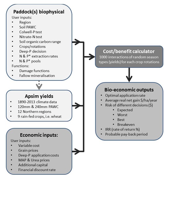
Figure 1. Schematic of the bio-economic framework of long-term decisions of deep-P placement using APSIM® and Excel®
Deep-P bio-economic framework thresholds
Based on previous analysis, we have assumed that soil will be deep-P responsive when Colwell P is <10 mg/kg and BSES P is < 30 mg/kg in the 10‐30cm layer, and that the residual benefit of deep bands will occur if the PBI is < 200 (Bell et al., 2014). Of course, a soil test below this threshold does not guarantee a crop response, and therefore should be used as an indicator of a probable response.
In this study we have assumed that 1 mg/kg Colwell P represents 1 kg plant-available P/ha in a 10cm layer, and that each kg of crop P removal is equivalent to 1 mg Colwell P/kg extracted across the crop root zone. However, we know from previous research that >90% of that net removal comes from the top 30cm of the profile, with roughly half from the 0-10cm and the other half from the 10-30cm layers. The 10-30cm soil test layer represents two soil bands 10cm thick (10-20 and 20-30 cm), therefore the amount of P in that layer is twice the soil test value (called P* in the set-up).
There is little historic data in the NGR on responses to deep P for any crops – other than what we have generated in the last few years (Bell et al., 2014). Therefore we have used three basic season types, with characteristics that influence crop response to deep P, as suggested by Bell et al. (2014):
- Dry start – those years with little or no effective rainfall from planting until after tillering;
- No stress – no severe crop stress, with an expectation that more regular rainfall will ensure the top soils have plenty of active roots; and
- Late stress – those with enough rain to ensure good early growth, secondary root development and tillering but serious later water deficits that ensure a strong reliance on subsoil moisture.
Case study
The case study is based on a paddock in the Goondiwindi region, producing sorghum, chickpea and wheat, on soil with a PAWC of 180 mm, nitrate-N of 50 kg N/ha, soil organic carbon between 0.85 and 0.95%, Colwell-P soil test in the 10-30 cm of 5 mg/kg, and PBI of 100, meaning the soil is very likely to be P responsive. We compared the risks and benefits of applying a low rate of MAP at depth for a 3-year “short-rotation” of sorghum, chickpea, wheat, wheat crops against a higher rate of MAP for a 7-year “long-rotation.”
The climatic records (1890-2013) from Goondiwindi were used to estimate season types and to run APSIM for yield distributions for soils of 120 and 240 mm PAWC. The bio-economic framework is designed so that any PAWC can be selected between 120-240 mm, using a linear regression between these two values.
Inputs for our case study site (Table 2 and below):
- Deep-P placement is by a currently owned John Deere® 8400 tractor and planter attachment set at a soil-depth of 200-250 mm. The cost includes fuel, oil, repairs, maintenance, efficiency losses, and additional depreciation based on machinery hours totalling $31.58/ha.
- Deep-P placement will result in increased yields and therefore 10% more N will also be placed in shallow soil layers for sorghum and wheat crops at a cost of $800/t.
- MAP (P = 22%) is used for the deep-P application at a cost of $730/t.
Table 2. Input criteria relating to P and N removed, the yield benefit from applied deep-P (from Bell et al. 2014) and crop-related costs and prices
|
|
Nutrients removed from soil by crops (kg/ harvested t) |
Damage (discount) to crop when Colwell-P<10mg/kg (P*<20kg/ha) |
Variable costs |
Farm gate prices |
||||||
|---|---|---|---|---|---|---|---|---|---|---|
|
Crop |
120mm PAWC |
240mm PAWC |
||||||||
|
P* |
Net N |
Dry start |
No stress |
Late stress |
Dry start |
No stress |
Late stress |
$/ha |
$/t |
|
|
Chickpea DC |
3.8 |
0 |
5% |
10% |
15% |
30% |
10% |
25% |
342 |
409 |
|
Sorghum LF |
2.3 |
17 |
5% |
15% |
10% |
10% |
15% |
25% |
462 |
230 |
|
Wheat |
2.6 |
23 |
5% |
15% |
10% |
10% |
15% |
25% |
319 |
257 |
When dealing with long-term investments we need to consider the opportunity cost of not investing the money elsewhere or financing. We do this by discounting future cash flows to a net present value (NPV). The discount rate will be different for different people based on their opportunity costs, cost of finance, and/or compensation for undertaking the risky venture. In our analysis we have assumed that this deep-P venture will use bank financing and added risk, so the farmer will need to receive 10% p.a. for the duration of the crop rotation. However, when you have long-term investments of different time horizons, the analysis will bias towards the longer-term investment due to longer cash flows. Therefore, to compare these projects we need to convert NPVs into annuities, we call this the annual net benefit ($/ha/year). This is basically the current value of additional income per year over the project life, i.e. the farmer should be indifferent if they received the lump sum NPV or if they received the annual amounts. Although the first crop is long-fallowed, the investment horizon of deep-P will start at the time of application just prior to planting.
Another long-term investment measure is the internal rate of return (IRR) which is basically the return on investment for long-term investments represented in % p.a. Any P* depleted from or left in the soil after this point has been ignored. This deep-P framework is meant to be used in a stepwise fashion through time, in that after a few seasons another Colwell test is needed to evaluate if there is still sufficient P* and if it is economical to replenish the P* pool, this likely after consecutive high yielding years.
Results
Returns vs risk
The calculator is able to determine the optimal P fertiliser rate and the annual net benefits of applying the deep-P compared to nil applied deep-P. The calculator also measures the risk associated with the alternative deep-P strategies. Based on these findings a farmer may opt for a lower risk and expected-return or vice-versa based on their risk preference.
Optimal P fertiliser rate
Based on the expected (median or 50 percentile) outcomes, the optimal deep-P application rate for the short and long rotations used in the case study are approximately 135 kg/ha and 270 kg/ha of MAP respectively as shown by the maximum point on median line and the annual net benefits (Figure 2).
Comparison of net benefits over the short and long rotation
The maximum median annual net benefit was $43/ha/year and $76/ha/year in the short and long rotations respectively.
Under the worst-case scenario (0 percentile), being a series of poor seasons, the optimal application rate for the long-rotation did not change but resulted in the annual net return of only $6/ha/year; however, for the short-rotation the optimal rate decreased by 34 kg to 101 kg/ha MAP and resulted in a loss of $9/ha/year.
Under the best-case scenario (100 percentile), rain when you want it, the optimal application rate increases to 338 kg/ha MAP for the long-rotation, with an annual net benefit of $150/ha/year. That is, increasing MAP application by 68 kg/ha it is possible to get an extra $11/ha/year with exceptionally good run of seasons but this amount of MAP would be excessive for all other seasons.
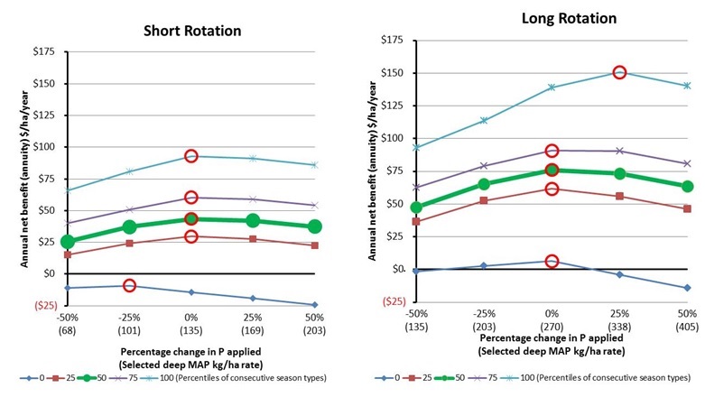
Figure 2. The real annual net benefit of deep-P (MAP) placement of a short and long rotations with respect to different seasonal outcomes: percentile = 0 is the worst-case scenario, 100 is the best case, and 50 is the expected outcome. The red circles indicate the optimal application rate for the given seasons.
Quantifying the risk and variability of potential outcomes
Assuming that the farmer is risk neutral and the optimal decision is to maximise the expected value, the annual returns will be between -$14 and $93/ha for the short-rotation and $6 and $139/ha for the long-rotation. These distributions are one measure of risk. Although not graphically presented here, the framework reported a 7% probability of not breaking even for the short-rotation, the long-rotation was almost certain to breakeven. The framework also showed that the long-rotation was always better (stochastic dominance) over the short-rotation, meaning that it will always result in a higher annual net return.
Effect of deep-P on crop yields and net benefit over time
The calculator quantifies the median change of yields and net benefits over the example rotations (Table 3). The cumulative crop length (years) indicates the time series of the proposed rotation.
There are three streams of expected (median) yields from each of rotations: unconstrained (APSIM) without any penalties from insufficient nutrients, yields with added deep-P and starter P, and no applied P. The lower net benefit with both rotations in the first season is due to the cost of deep-P application, which proves that it is a long-term investment over multiple seasons.
Table 3. Yield and economic output from the economic framework calculator
Long rotation
| Sorghum LF |
Chickpea DC |
Wheat |
Wheat |
Sorghum LF |
Chickpea DC |
Wheat |
Wheat | |
|---|---|---|---|---|---|---|---|---|
| Cumulative crop length (years) |
0.4 | 1 |
2 | 3 | 4.4 |
5 |
6 | 7 |
| Yield (kg/ha) unlimited N & P |
4,654 |
1,359 | 3,266 |
3,210 |
4,654 | 1,313 | 2,988 | 3,081 |
| Yield (kg/ha) with added P |
4,654 | 1,359 |
3,266 |
3,210 | 4,654 | 1,313 | 2,975 | 2,922 |
| Yield (kg/ha) without added P |
4,082 | 1,169 |
2,730 |
2,715 | 3,943 | 1,076 | 2,528 | 2,550 |
| Net benefit of P treatment |
-$132 | $86 | $122 | $124 | $144 | $86 | $113 | $70 |
Short rotation
| Sorghum LF |
Chickpea DC |
Wheat | Wheat |
|
|---|---|---|---|---|
| Cumulative crop length (years) |
0.4 | 1 | 2 | 3 |
| Yield (kg/ha) unlimited N & P |
4,654 | 1,359 | 3,266 | 3,210 |
| Yield (kg/ha) with added P |
4,654 | 1,359 | 3,266 | 3,081 |
| Yield (kg/ha) without added P |
4,082 | 1,169 | 2,730 | 2,715 |
| Net benefit of P treatment |
-$33 | $86 | $121 | $108 |
Return on investment on deep-P
The other consideration for long-term investments is the return on investment was well as the payback period of the initial investment. The internal rate of return (IRR) for the short- and long-rotation is 142% and 67% p.a., which is far greater than the opportunity cost of 10% (Figure 3). Although the annual returns of the long-rotation are higher under all situations, the expected (median) IRR is lower due to the higher initial financial investment. However, the risk (uncertainty) associated with the short-rotation is also far greater. Under the worst-case scenario it is possible to have an -18% IRR and there is a 5% chance of getting a negative IRR. The higher risk of the short-rotation is also indicated by the high IRR under the best-case scenario of 750% compared to the long-rotation 224%. In summary, the long-rotation IRR is lower, but it is more predictable (less variable) and is almost guaranteed to have a positive IRR. Although not shown, the short- and long-rotation has about an 85% chance of getting >10%, which is the opportunity cost.
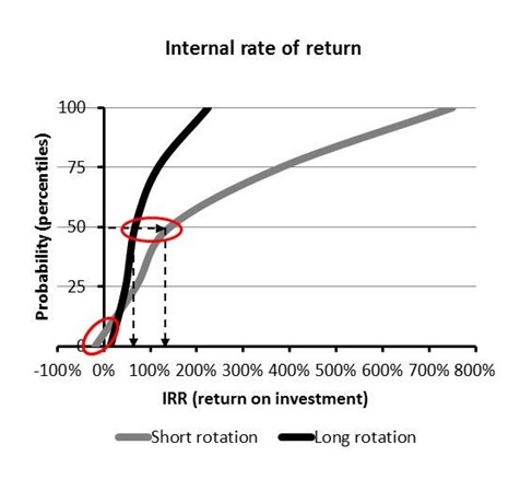
Figure 3. The distribution of internal rates of return for the short- and long-rotation option: percentile = 0 is the worst-case scenario, 100 the best case, and 50 the expected.
Payback period
The expected payback period of both the short- and long-rotations is two-years (Figure 5). However there is a greater probability of the short-rotation decision being paid back sooner due to the low rate of deep P, hence lower initial investment of the short-rotation. There is a 1% chance of never receiving a payback. Under the worst conditions the cost outlay for fertiliser in the long-rotation is expected to be paid pack in the fifth year.
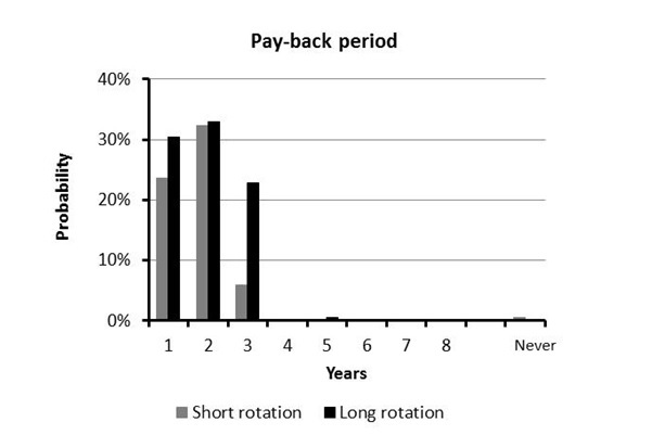
Figure 4. The frequency of which the initial investment is paid back in a particular year. “Never” indicates that it was never fully paid back.
Discussion
The decision to apply deep-P is different to most fertiliser decision because it involves a single high application of fertiliser product that is hoped to supply financial benefits over a number of seasons for which future climatic conditions and starting soil moisture are unknown. Hence several technical and economic factors need to be included in the analysis.
The decision to apply deep-P has the following considerations that this economic framework (calculator) can address;
1. Is deep P required?
- The framework uses best current research knowledge of critical soil levels, and predicts whether it is likely to be worthwhile proceeding with a deep-P application
- P application rates can be varied to find the optimum P rate for the highest financial return.
- Once the optimal rate is identified based on the expected annual net returns for the different crop rotations, then the grower needs to assess the risk: best- and worst-scenario.
2. What is the optimum deep-P rate to apply for a given time horizon?
3. How much P, how often and what is the risk?
4. What is the internal rate of return and payback time?
- For added information about risk and financing, graphs are presented on returns on investment and payback period of different deep-P decisions.
The framework can be used to examine the cost/benefit trade-offs of deep-P decisions over time and the implications of expected prices, costs and crop rotation practices.
It demonstrates the potential yield benefits of correcting P deficiencies at depth, as well as the costs and cash-flow implications that may be involved.
Moreover this framework can also be used by farmers to communicate the potential returns and even the risk (worst-case scenarios) to financial institutions, when seeking additional finance.
The case study of different application rates is only one example for which this framework could be used. It can also be used to investigate the returns and risk with respect to different levels of Colwell-P measurements, soil PAWC, different paddocks on a farm, changing input and output prices and even other long-term amelioration or nutrient decisions.
References
Bell, M., Lester, D., Power, B., Zull, A. F., Cox, H., McMullen, G., & Laycock, J. (2014). Changing nutrient management strategies in response to declining background fertility: The economics of deep Phosphorus use. Paper presented at the GRDC Grains Research Update: Goondiwindi.
Acknowledgements
The research undertaken as part of this project is made possible by the significant contributions of growers through both trial cooperation and the support of the GRDC, the author would like to thank them for their continued support.
Contact details
Andrew Zull
Queensland Dept. of Agriculture, Fisheries and Forestry: Crop and Food Science
203 Tor St, Toowoomba, Qld. 4350
07 4688 1407
Andrew.Zull@daff.qld.gov.au
Was this page helpful?
YOUR FEEDBACK