Adjusting the enterprise mix for 2017 and beyond
Author: David Crowley (Delta Agribusiness, Young and Quandialla). | Date: 02 Mar 2017
Take home messages
- Strong livestock markets and flat cereal grain prices are influencing the enterprise mix on many farms across southern NSW.
- Significantly changing the enterprise mix to include more livestock may have negative cash flow consequences in the short to medium term.
- Before making major changes to the enterprise mix, long term average production potential and projected commodity prices must be carefully evaluated relative to individual passions and capabilities.
Background
The combination of buoyant livestock prices, a soft cereal grains market (despite mostly good yields), and variable canola yields provides adequate reason to re-assess the enterprise mix on many farms across southern NSW. Any adjustment, however, must be planned rather than reactionary, and subsequent business impacts should be considered across several seasons. In most cases, adjusting the enterprise mix will impact business cash flow, profit and risk position.Re-evaluating the proportion of crop versus livestock in the farming system has arisen due to the increased frequency of more variable (or extreme) seasonal conditions that have occurred over the past decade. Whether these conditions are frost, dry/droughted springs or excessive wet weather, the stability of livestock income has often been noted throughout. Consequently, many producers have contemplated or are contemplating reducing the percentage of the farm sown to crop and increasing livestock numbers. This is because livestock are less costly and perceived to be less risky year in, year out, and more recently, livestock returns are rivalling or surpassing those of long term cropping averages.
Case study: adjusting the enterprise mix 2017-2021
The following case study has been put together to demonstrate the impact of reducing crop area and increasing livestock numbers on both business cash flow and whole farm profitability over a five year period.
The principles applied here will be common to many farms within the region, however, while every effort has been made to ensure the accuracy of the numbers used, the case study provides a general overview only and will differ on an individual basis. Before undertaking any course of action, please talk to your local adviser.
To examine this shift in enterprise mix, a mock 1,200 hectare (3,000 acre) farm under two scenarios has been examined:
Scenario 1
- 1,200ha with 60% crop and 40% pasture as a constant balance. The crop is a mix of wheat and canola with approximately one-third of this area sown to canola. The pasture area (40%) is dedicated to running a self-replacing 21 micron merino flock, which joins 25% of ewes to terminal sires. The stocking rate has traditionally been maintained at 8.0dse/ha with a flock of 1,800 ewes.
- Crop/pasture area is kept constant at 60% crop, 40% pasture by sowing two 40ha paddocks to pasture (undersown) and bringing two paddocks out of pasture back into the cropping rotation each year.
Scenario 2
- 1,200 ha shifting from Scenario 1 to 40% crop and 60% pasture. The aim here is to reduce exposure to the variable returns of cropping and to increase ewe numbers by retaining more ewe lambs
- To shift to less crop and more pasture, only one new paddock of crop will be brought into the rotation each year and three paddocks will be undersown (compared to a balance of two paddocks in and two out annually in Scenario 1).
- Ewe numbers will be increased by 300 each year (until they reach 2,700) by retaining more ewe lambs.
- The 1,200 ha farm begins with 83% equity, which means it has $770,000 of land and machinery related debt, and an existing overdraft of $100,000.
- The land is valued at $3,706/ha ($1,500/acre).
- Carrying capacity of the perennial pasture area is 8dse/ha.
- Wheat and canola prices are stable across the five year period at $200/t and $500/t, respectively (local silo).
- Ewe lambs are sold for $150/head and wether lambs are sold for $120/head.
- Wool price is $1,400c/kg clean (a substantial increase on previous seasons).
- Pastures are lucerne based, combined with a mix of annual clovers.
- Half the pasture area will be top-dressed with single super each year.
- 80 tonnes of barley are purchased at $180/t for supplementary feed. This quantity increases incrementally to 130 tonnes by 2021 in Scenario 2.
- Lambing % = 90%.
- $80,000/year is allocated to drawings/managerial expenses.
- Profit is defined as gross income less overheads, variable costs, depreciation, interest payments and an allowance for drawings.
- Long term average crop yields are used to account for seasonal variability year on year (yields assumed the same for both scenarios).
| Crop | Yield | Gross Margin ($/ha) |
|---|---|---|
| Wheat on Canola | 3.5t/ha | $346 |
| Wheat on Wheat | 3.3t/ha | $293 |
| Wheat Undersown | 2.3t/ha | $118 |
| Canola | 1.6t/ha | $378 |
| Merino x 25% Terminal | 8.0dse/ha | $482 |
Results and discussion
Figure 1 highlights the difference in farm profit generated over a five year period between the two scenarios. The light grey line represents a maintained 60:40 crop/pasture farm breakup, and the thick black line shows what happens when the second scenario is adopted and the enterprise mix changes from 60:40 crop/pasture to the reverse (Scenario 2).
In Scenario 2 (the thick black line), farm profits initially decline as more paddocks are undersown, less area is cropped and less ewe lambs are sold because more are being retained for joining. It could be argued that the gap between these two scenarios would be greater in a year when higher crop yields were attained and slightly closer together when crop yields were poor. However, it should not be forgotten that in a poor cropping year (a dry spring) stock margins will also likely be tighter due to increased supplementary feeding and lower lamb prices.
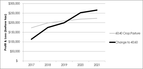
Figure 1. Farm Profit and Loss (P&L).
Even when long term livestock gross margins are significantly higher than those of crops, it takes three years for the farm business profits to reach a point where the change to more livestock becomes more profitable than maintaining the original status quo. This can be attributed to retaining more ewe lambs for joining rather than sale, and a larger proportion of wheat undersown (lower crop gross margins) in the mix. Simply because livestock may have the potential to produce a higher gross margin than cropping (on current market values), this does not mean that changing the enterprise mix will be immediately more profitable for the overall business. Moreover, the strength of the livestock gross margins is generated by maximising carrying capacity which can only be done by maintaining a strong perennial pasture base.
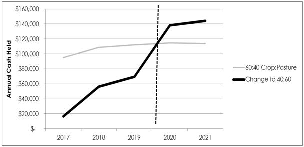
Figure 2. Annual cash held.
The change in profit does not, however, explain the whole impact of the change in enterprise mix on the business. As the enterprise mix moves to less crop (40%) and more pasture (60%), the annual cash held (the amount of money left over at the end of the year after all business activities have taken place) declines as the crop area is reduced and while more ewe lambs are being retained to increase ewe numbers. Note that this trend improves as ewe numbers become stable in 2020, but cash flow is significantly hampered as the change takes place. This represents the cost that is incurred by the business by making the change.
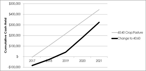
Figure 3. Cumulative cash held.
Cumulative cash held (Figure 3) represents what would happen if all profits are kept within the business and are not spent updating machinery or farm infrastructure. For the sake of simplicity and easy comparison, there has been no principle paid off the land related debt. However, the overdraft level which starts at $100,000 is reduced as funds become available. Note that in the process of changing to the second 40:60 crop/pasture scenario, because cash on hand becomes tighter during the transition period, the $100,000 overdraft is maintained, whereas in the first scenario when the rotation remains static, the overdraft can be paid out in the first couple of seasons.
At the end of the five year period, the 1,200ha case study farm would have been approximately $120,000 better off by staying with 60% crop, 40% pasture break up, assuming that the average yields can be consistently achieved during the five year period. Further, when examining this result, it must be noted that the wheat price used for this model (wheat @ $200/t local silo) is on the lower end of historical price deciles, while lamb and wool prices are historically high (Table 2).
Table 2. Commodity deciles June 2007-2016.
From Jul-07 to Jun-16
| Percentile | 17.5 | 19 | 21 | Trade Lamb c/kg dwt |
Mutton c/kg dwt |
Steers c/kg lwt |
Cows c/kg lwt |
Wheat ASW |
Canola |
|---|---|---|---|---|---|---|---|---|---|
| c/kg clean | |||||||||
| 100% | 2275 | 1772 | 1526 | 690 | 504 | 349 | 260 | 490 | 800 |
| 90% | 1606 | 1468 | 1340 | 574 | 411 | 283 | 199 | 336 | 620 |
| 80% | 1463 | 1390 | 1281 | 532 | 375 | 217 | 150 | 310 | 580 |
| 70% | 1371 | 1294 | 1214 | 510 | 340 | 208 | 144 | 296 | 565 |
| 60% | 1323 | 1238 | 1154 | 486 | 313 | 200 | 139 | 284 | 546 |
| 50% | 1276 | 1197 | 1098 | 466 | 282 | 195 | 135 | 278 | 533 |
| 40% | 1240 | 1145 | 1000 | 432 | 234 | 190 | 132 | 270 | 515 |
| 30% | 1197 | 1101 | 954 | 400 | 194 | 184 | 129 | 257 | 500 |
| 20% | 1173 | 1056 | 885 | 367 | 169 | 178 | 125 | 229 | 480 |
| 10% | 1141 | 987 | 788 | 329 | 141 | 170 | 120 | 200 | 435 |
| 0% | 1006 | 887 | 672 | 181 | 18 | 152 | 95 | 172 | 390 |
| Av. 2015/16 | 1447 | 1408 | 1343 | 547 | 339 | 317 | 228 | 273 | 536 |
Nearest percentile to 2016 price = light grey shaded box
**Wheat and canola prices delivered port
Source: Andrew Woods, Independent Commodity Services.
Once the enterprise changeover has taken effect, the 40/60 Crop/Pasture model (Scenario 2) produces approximately $43,300 more profit year on year. Each individual business must then weigh this increase profit against the reduced exposure to risk or reward forgone in the cropping enterprise, and the impact of enterprise shift on business cash flow and liquidity. This must also be balanced against seasonal variability relative to farm location and the existing financial obligations of each individual business. For example, in an area which has received three major grain frosting events in the past 10 years, the arguably less volatile income produced in Scenario 2 may be deemed a more attractive outcome. Conversely, in areas predisposed to flooding, major damage to perennial legume pastures may shift the enterprise desirability back towards an increased proportion of crop.
Conclusion
Assuming commodity prices remain similar to those used in this analysis, reducing the area of the farm sown to crop and increasing livestock numbers will eventually be more profitable. However, cash flow and whole farm profit are reduced for three years, while the shift in enterprise mix takes place. Therefore, before making major changes to the enterprise mix, each individual business must assess its current equity and cash flow position.
This case study does not factor in good and bad years, but is presented on averages. It is designed to show the impact of a major enterprise mix shift on business profitability. Once the enterprise mix has changed and comparative earnings potential is realised, it is then up to the individual to assess whether the perceived lower level of risk with less crop in the system justifies the earning potential across seasons. Before undertaking any major enterprise mix shift, business health and long term enterprise profit/volatility must be objectively assessed and further evaluated relative to individual passions and capabilities.
Acknowledgements
Andrew Woods, Independent Commodity Services.
Cameron Rosser, Delta Agribusiness Livestock and Property.
Contact details
David Crowley
Delta Agribusiness
287 Boorowa St Young, 2594
(02) 63826622
dcrowley@deltaag.com.au
@davecrowls
Was this page helpful?
YOUR FEEDBACK