Profit drivers in the Lakes district of Western Australia – a case study
Author: Steve Curtin (ConsultAg) | Date: 13 Feb 2019
Take home messages
- A basic understanding of key business ratios is necessary to benchmark your business. There are three main drivers to profitability in any farming business – yield, price and expenditure.
- Yield for both cropping and livestock enterprises is the most important driver of profit.
- Key ratio long term trends are important in identifying the main changes required for farm enterprises as they respond to changing seasons and commodity prices.
- Farm operating costs have risen over recent years, but reasonable to good seasonal conditions have meant farm incomes have increased also. Consequently, businesses are recording good profits and have improved their financial position.
- In the Lakes area of Western Australia, farming businesses are performing just as well financially as Northern and Central wheatbelt farmers despite more adverse seasonal impacts such as drought and frost.
Background
The Lakes area of Western Australia is a farming district with distinct characteristics distinguishing it from other farming areas within Western Australia. ConsultAg consultants have many clients in this area and each year clients are analysed for their Client Averages Report which enables them to compare their business with others in the same environment and season. The report enables farmers to identify key areas where they are not performing and make changes if needed.
The main financial parameters for farmers to focus on when analysing their business are profitability, equity and liquidity. The relevant numbers in any one year are not as important as the trend over time. These three measures collectively provide insight to any business and all three should be performing well to confirm your business is making progress. The results presented in this paper summarise 10 years of data from 2007 to 2017 for 38 farm businesses. From this data it can be seen how farmers, and the area as a whole, have responded to seasonal influences, commodity prices, crop and enterprise choice and variety improvements. All with the aim of improving profitability.
An Annual Financial Review is the best way to measure the performance of any farming business. Any analysis will need a Cash Flow Budget (liquidity), Statement of Position (assets, liabilities and equity), and Profit Analysis including calculation of the Return on Capital (ROC).
Cash Flow Budget and Statement of Position are discussed in more detail in Appendix 1.
Profit analysis
Profit is the income left over after all operating, personal, depreciation and financing costs are covered. The amount remaining is referred to as Profit or Earnings Before Interest and Tax (EBIT) which is used to pay the tax bill, reduce debt or pay for capital items such as farm land, plant or off-farm investment. Table 1 shows a basic calculation for Profit. Farm operating costs are 58% of Income at $1,900,000. EBIT allows a business’s profit to be compared with other businesses without consideration for the costs of borrowing which can vary widely between farmers. EBIT is then used to calculate the Return on Capital (ROC). In this case if the farm has total assets of $10,000,000 then the ROC would be 9% ($900k/$10m).
Table 1. Basic Profit calculation.
| Total Farm Income $3,300,000 | |||
|---|---|---|---|
| Variable Costs 1,700,000 | |||
| Overheads 200,000 | |||
| Total Farm Operating Costs 1,900,000 | |||
| Farm Operating Surplus 1,400,000 | |||
| Drawings Actual 220,000 | |||
| Machinery Allowance 160,000 | |||
| Farm Lease 120,000 | |||
| Farm Profit or EBIT (before interest & tax) $900,000 | |||
| Interest Costs $200,000 | |||
| Farm Profit or EBT (before tax) $700,000 |
With the basic parameters of farm analysis established, it is possible to look in more detail at trends within the Lakes farming district of Western Australia over the last 10 years. A recent analysis for the Australian Association of Agricultural Consultants (WA) (AAAC (WA)) also compared trends over time for the Lakes area and the Northern and Central wheatbelt areas. This is discussed in this paper within the Comparison with other areas section.
Results and discussion
A selection of key ratios from 10 years of client averages was used to analyse trends within the district and to identify the key drivers of profit for farming businesses. This is particularly relevant in an environment of ever-increasing farm costs and current relative high commodity prices. The selected data is detailed in Appendix 2. Table 2 summarises some of the key ratios over the 10 year period and the more recent five year period since 2013.
Table 2. Key farm ratios (2007-2917).
Ratio | Average (10 yr) | Average (5 yr) | Range over 10 years |
|---|---|---|---|
Farm income ($/ha) | $372 | $446 | $191 - $487 |
Operating costs as % of Income | 71% | 62% | 49 - 106% |
Yield Wheat (t/ha) | 1.77 | 2.06 | 0.72 - 2.4 |
Profit ($/eff ha) | $37 | $88 | -$100 - $162 |
Stocking Rate (DSE/wgha) | 3.5 | 3.43 | 3.2 - 4.1 |
Return on Capital % | 4.7% | 7.9% | -5.2 – 15.1% |
Lambs % | 84% | 88% | 76 - 91% |
Wool (kg/wgha) | 15 | 16.7 | 9 - 18.6 |
Profit and Return on Capital (ROC)
Profit is about margin. It is the difference between the income received and the amount spent to achieve that income. Expenditure includes all operating costs and overheads, personal costs, lease and machinery depreciation.
Profit (EBIT) can then be spent on debt repayments (including machinery financed), interest and off farm investments.
Profit has varied widely over the last 10 years depending on seasonal influences; ranging from -$100/ha in the drought years to $162/ha in the good years (Figure 1). An average of $37/ha includes all years with droughts and frosts but hides the recent performance of farms in the area since 2013. Since then the five-year average is $88/ha.
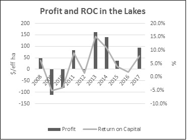
Figure 1. Profit ($/effective ha) and Return on Capital (%) in the Lakes area of WA
Most businesses are a mix of crop and livestock enterprises with 75% having sheep as their livestock choice. Mixed farming enterprises still have a high proportion of their profit as cropping income. The average was 82% crop income despite the recent high sheep and wool prices. Income % from cropping ranged from 74-91% depending on the season. Sheep income was higher in the poorer cropping years of 2010 and 2016.
The ROC has averaged 4.7% over 10 years but in the last five years has risen to 7.9% and shows the influence of better seasons since 2013. In the previous five years the ROC was a dismal 1.5%.
Yield
Yield remains the main driver of profitability that farmers have control over. Yields have been steadily increasing over the last 10 years. Figure 2 shows the rolling three-year average for wheat and barley yields. For the first time in this area, wheat has achieved a five-year average yield higher than 2t/ha. This would have been unprecedented 10 years ago.
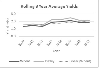
Figure 2. Cereal yields over a rolling three-year average.
The Lakes area has shown a 9% decrease in growing season rainfall (GSR) over the last 10 years decreasing from 250mm to current average of 223mm. At the same time there has been an increase in efficiency of wheat production from 6.5 to 9.2 as measured by kg/mm GSR. Farmers have actively stored any summer moisture with stubble cover retention and weed control, dry sown crops and incorporated other practices which have allowed them to be more efficient in utilising rainfall and stored moisture. Wheat yield increase due to variety has not been a major factor over time, but barley varieties have improved substantially in the last 10 years. Combine that with improved agronomic practices regarding fertiliser and disease management and yields have been lifted overall, allowing farmers to keep up with rising costs.
Price obviously has also a big part to play in determining profit, but farmers have no control over the market other than to make sure that grain is sold at a price which makes a profit.
Figure 3 shows the relationship between yield and profit and indicates that there is a good relationship. The message is clear that farmers should focus their efforts on maximising yields.
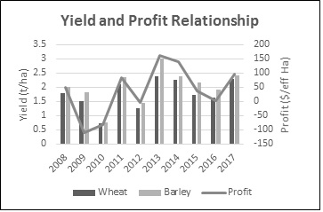
Figure 3. Relationship between yield and profit over 10 years.
Price
The prices received for grain and livestock have an influence on profit but as mentioned previously are not the main determinant of profit. Figure 4 shows the relationship between price and profit and indicates that it is a poor relationship.
Certainly, price makes the good yielding years better but does not have as much impact on profit in the poorer yielding years. The data suggests that a focus on yield provides the best return for your effort followed by price.
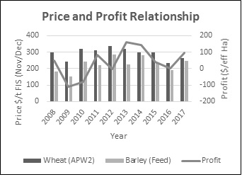
Figure 4. Relationship between price and profit (2008-2017).
This is not saying farmers should not have a marketing plan or stay aware of prices. Quite the contrary. All farming businesses need to know the price at which they make a profit at any level of yield. This is usually done at budget time each year when average yields and long-term prices are used to produce a Cash Flow budget. This takes into account yield, price and expenses of the business. Analysis can then be carried out to determine the price level at which a desired and reasonable profit is produced. A reasonable guide should be at least 5% ROC. This then allows the business to lock in a profit if/when these prices are achieved during the season depending on production expectations as the season unfolds. It also takes away any uncertainty as to what is a good price or not.
Sheep and wool prices have improved markedly over the last 10 years and have had a big impact on sheep profitability. Figures 5 and 6 show the prices of wool (WMI) and two different classes (trade lambs and mutton) of livestock (MLA) over the last 10 years and show that prices have doubled over that time.
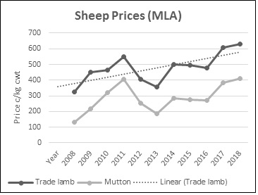
Figure 5. Livestock prices (cents/kg cwt) over 10-year period (Source: MLA).
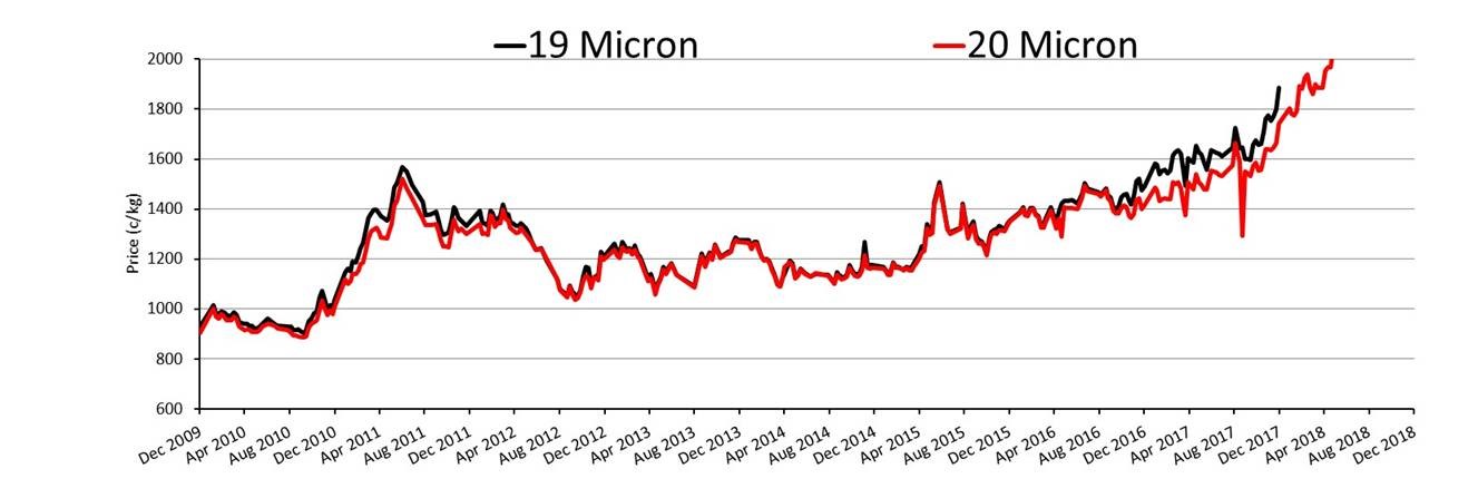
Figure 6. Wool Prices (Net sweep the floor cents/kg) over 10 year period (Source: WMI).
Price has also influenced how efficiently farmers run their sheep and even the type of sheep they run. Recent better prices have encouraged farmers to put more effort into livestock production with a corresponding lift in key production ratios as outlined in the section on Enterprise trends. But the same applies to livestock as cropping. Get the yield per hectare right first and price second.
Operating Costs
Expenditure is the third component which impacts profit. How much of this expenditure is yield increasing and how much is not necessary, is important to identify.
Figure 7 shows the increase in Operating Costs over the last 10 years. Income is included also and it can be seen that, despite the increase in costs, farm income (yield by price) has kept pace. Operating costs as a % of income has averaged 71% over 10 years and 62% over the last five years which have been better seasons.
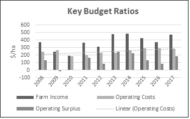
Figure 7. Farm Income, Operating Costs and Operating Surplus over 10 years.
Essential items which consistently increase in budgets are inputs such as fertiliser, chemical, fuel, repairs, labour and more recently stock expenses. Table 3 highlights the percentage increase of three selected items of Operating Costs calculated from a rolling three-year average to even out any extreme years. The actual dollar amount cost increase is shown as well as the increase as a percentage of operating costs. This shows a smaller relative increase because all costs are increasing.
Table 3. Increase in selected expenditure items from Operating Costs over a 10 year period (2007 – 2017).
| Repairs ($/crop ha) | Stock Expenses ($/pasture ha) | Labour ($/effective ha) | |
|---|---|---|---|
| 3 Year Average (2017) | $32.70 | $124.50 | $20.70 |
| Increase ($/ha) | 46% | 50% | 86% |
| Increase (% Op costs) | 17% | 20% | 49% |
One measure of efficiency that hasn’t changed over the years is labour productivity. Tonnes of grain produced/labour unit has remained around 2,500t/labour unit and shows good utilisation of available labour. It is the cost of labour that has increased over the time period.
While costs have increased substantially in terms of $/ha , the actual increase as a % of Operating Costs is a smaller amount. Using a similar analysis, the dollar amount of drawings or personal expenditure has increased by 29% over the last 10 years, but as a % of Income it has actually dropped by 32%. This highlights the increase in income from the more favourable seasons in recent years
Return on Capital
Return on Capital (ROC) is a key measure to ensure the business is making enough profit to invest in further expansion, off farm assets and pay down debt. Farms with profitable leases usually generate higher returns as the land is not included as an asset. However, the amount of leased land has not grown over the 10 year period indicating the amount of leased land available is reasonably constant. What has grown substantially for the Lakes area is land ownership over the last 10 years. This is due in part to the better seasons since 2013 and resulting profitability of farming in the area. As land has become available it has been competitively sought after by neighbours and outsiders keen to increase their holdings. Figure 8 shows that average arable area farmed has increased from 3,800ha 10 years ago to 4,600ha – an increase of 21%. This is in strong contrast to other farming areas which have undergone more modest area increases.
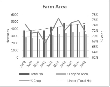
Figure 8. Total area owned and area cropped
This increase in area farmed has also meant that there has been a substantial upgrade in machinery capacity over the last 10 years. In 2008, machinery ownership was $288/cropped ha. In 2017 it was $499/cropped ha and has averaged $436/cropped ha over the last five years since the run of good seasons starting in 2013. The Lakes area has finally caught up to the Central and Northern wheatbelt areas.
Enterprise trends
With the change in prices, improvement in barley yields and the increased level of risk from climatic factors such as frost, there has been a change in enterprise mix over the last 10 years in order to reduce risk and maintain profitability.
Cropping
The Lakes area has seen a change in cropping mainly from wheat to barley. This is due to barley’s higher yield potential through improved varieties and its relative safety under frost prone conditions compared to wheat. Farmers are now sowing it as a primary crop in the rotation rather than a secondary crop after wheat.
Barley is also able to be sown earlier and so takes the place of early sown wheat which is a high frost risk. Wheat now takes up 40% of cropped area compared to 60% 10 years ago. In the same time barley has increased from 20-25% to 35% of cropped area. Alternative crops such as canola and lupins have remained consistent at 8-9% of cropped area.
Sheep
Seventy-five per cent of farmers in the Lakes area still utilise sheep as an enterprise option. Sheep have a lower input cost compared to cropping and have minimal seasonal risk especially at the conservative stocking rates being run.
Figure 9 shows the change in flock composition over the last 10 years which can mainly be attributed to increases in both meat and wool prices. Less farmers are running crossbreds now but those who still do, have increased their crossbred matings.
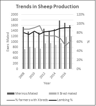
Figure 9. Trends in sheep production ratios.
There has been a 20% increase in merinos mated. Interestingly, with the higher prices, famers are now improving their sheep performance (yield) with lambing rates increasing from 80% to 90% and wool cut/winter grazed hectares (wgha) increasing by over 20% to 17kg/wgha.
A common question is whether sheep gross margins are now better than crop at current pricing. Although margins have increased by over 260% from $71/ha to $187/ha it is unlikely, given that cropping has also improved at the same time.
Figure 10 shows the steady increase in sheep income, costs and gross margins over the last 10 years.
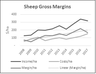
Figure 10. Sheep income, costs and gross margin.
Comparison with other farming areas
Figures 11, 12 and 13 compare the Lakes area with farms in the Central and Northern wheatbelts. It is obvious that we have had more production hiccups over the last 10 years but importantly, our strength is we have been able to keep operating expenses down compared to other areas. Part of this is the environment effect where we have less diseases and generally lower weed control costs. Looking at the important indicator of Operating Surplus it is clear the area is keeping up with other farming areas in all but the dry and frost impacted years.
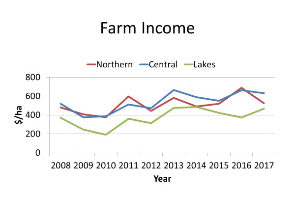
Figure 11. Farm income in different zones
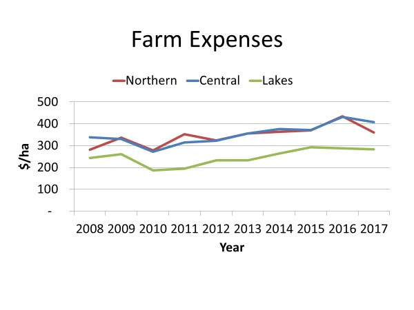
Figure 12.Farm expenses in different zones.
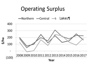
Figure 13.Operating surplus in different zones.
Conclusion
Despite the increase in costs over the last 10 years the increase in income has been able to keep pace. The combination of higher yield and prices and generally lower costs of production when compared to other higher input farming areas has allowed businesses in the Lakes area to return their businesses to a more secure level of equity which will help buffer them for the next poor season.
In summary
- Yield is still the main determinant of profit.
- Businesses have increased their scale of operation by increasing farm size which reduces overhead costs/ha. It has also meant a rush to acquire additional machinery capacity.
- Given the recent good position most farm businesses find themselves in, it is important not to get caught up in the euphoria of the Northern wheatbelt. Southern areas will still return reasonable profits due to good prices and it is critical that farmers be strategic in allocating any extra profits.
- Prioritise any profits to secure the financial position of the business to be able to take advantage of any future opportunities that may present.
Future opportunities for the area include more changes to enterprises to include chemical fallow, oats and hay for added diversity and lower frost risk and improvements in livestock management while sheep and wool prices remain high. In the Lakes area there has also been an increase in rejuvenation of ironstone and gravel soils with liming and reefinating which has brought previously problematic areas into production. This trend is set to continue.
Useful resources
ConsultAg client averages 2008-2018. Internal annual publications for ConsultAg clients
Contact details
Steve Curtin
sc@consultag.com.au
Appendix 1
Cash Flow Budget
The important items in the cash flow budget are the Operating Surplus and the Cash Surplus. Table 1 shows two different farms with different Operating Costs which determines the Operating Surplus. This then determines how much a business has to spend on the ‘other’ parts of the business. Once this is done the business is either left with a surplus (Farm A) or a deficit (Farm B).
Table 1. Summary of Cash Flow Budget for two farming businesses. Numbers represent cents in the dollar.
Farm “A” | Farm “B” | |
|---|---|---|
Income | 100 | 100 |
Operating Costs, Overheads | 60 | 75 |
Operating Surplus | 40 | 25 |
Drawings | 10 | 10 |
Tax | 5 | 2 |
Plant | 5 | 5 |
Finance | 10 | 10 |
Capital | 5 | - |
Off-Farm | 2 | - |
Cash Surplus/Deficit 3 -2 | ||
Liquidity
Good liquidity is the ability to pay for expenses when they are due or as the season dictates. It is access to funds or borrowing capacity. It allows businesses to take advantage of opportunities during the season and is necessary for long term growth. Figure 1 shows a business with good liquidity and Figure 2 represents a business with poor liquidity.
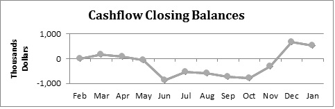
Figure 1. Working Capital $1m, Borrowing Limit $1.7m, Cash Surplus $500,000.
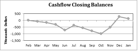
Figure 2. Working Capital $1m, Borrowing Limit $1m, Cash Surplus $128,000
Appendix 2
Table 2. Ten year summaries of selected ConsultAg Client Data.
Parameter | 2008 | 2009 | 2010 | 2011 | 2012 | 2013 | 2014 | 2015 | 2016 | 2017 |
|---|---|---|---|---|---|---|---|---|---|---|
Effective area farmed (ha) | 3,790 | 3,861 | 3,595 | 3,812 | 4,346 | 4,269 | 4,814 | 4,744 | 4,655 | 4,570 |
GSR (mm) | 320 | 203 | 115 | 280 | 142 | 236 | 312 | 199 | 214 | 204 |
Total crop hectares (ha) | 2,827 | 2,750 | 2,575 | 2,574 | 3,129 | 3,278 | 3,481 | 3,564 | 3,534 | 3,275 |
Livestock hectares (ha) | 963 | 1,111 | 1,020 | 1,238 | 1,217 | 991 | 1,333 | 1,180 | 1,121 | 1,295 |
Cropping % (% arable) | 75% | 71% | 72% | 68% | 72% | 77% | 72% | 75% | 76% | 72% |
Livestock area (% arable) | 25% | 29% | 28% | 32% | 28% | 23% | 28% | 25% | 24% | 28% |
Wheat (% ha cropped) | 54% | 58% | 59% | 60% | 51% | 50% | 47% | 46% | 39% | 38% |
Barley (% ha cropped) | 30% | 25% | 22% | 27% | 29% | 30% | 31% | 33% | 36% | 34% |
Canola (% ha cropped) | 8% | 11% | 11% | 10% | 13% | 15% | 14% | 13% | 13% | 13% |
Lupins (% ha cropped) | 8% | 11% | 8% | 8% | 10% | 9% | 9% | 8% | 9% | 7% |
Wheat yield (t/ha) | 1.8 | 1.52 | 0.72 | 2.11 | 1.25 | 2.39 | 2.26 | 1.73 | 1.62 | 2.3 |
Barley yield (t/ha) | 2 | 1.82 | 0.76 | 2.36 | 1.43 | 3 | 2.39 | 2.15 | 1.9 | 2.4 |
Canola yield (t/ha) | 1.2 | 0.77 | 0.28 | 1.03 | 0.69 | 1.42 | 1.16 | 0.87 | 1.11 | 0.7 |
Lupin yield (t/ha) | 1.1 | 0.85 | 0.26 | 1.41 | 0.67 | 1.89 | 1.4 | 0.86 | 2.18 | 1 |
Farm income ($/eff ha) | 372 | 247 | 191 | 361 | 314 | 477 | 487 | 424 | 374 | 468 |
Operating expenses ($/ha) | 243 | 261 | 187 | 195 | 232 | 232 | 264 | 293 | 288 | 283 |
% Operating Costs | 65% | 106% | 98% | 54% | 74% | 49% | 54% | 69% | 77% | 60% |
Operating surplus ($/eff ha) | 129 | -14 | 3.5 | 166 | 82 | 244 | 223 | 130 | 87 | 185 |
Farm assets ($/eff ha) | 1401 | 1794 | 1434 | 1539 | 1445 | 1565 | 1637 | 1554 | 1606 | 1709 |
Farm liabilities ($/eff ha) | 242 | 332 | 304 | 390 | 385 | 361 | 330 | 332 | 372 | 382 |
Equity (%) | 83% | 81% | 79% | 75% | 73% | 77% | 80% | 79% | 77% | 78% |
Profit (EBT/eff ha) | 48 | -111 | -81 | 82.2 | -4.24 | 162 | 141 | 37.75 | 2.95 | 95 |
ROC % (EBIT) | 6.1% | -5.2% | -4.0% | 9.0% | 1.5% | 15.1% | 10.9% | 3.8% | 1.8% | 7.9% |
T grain /labour unit | 2,527 | 2,345 | 2,310 | 2,767 | 2,614 | 2,414 | 2,469 | |||
Labour cost ($/crop ha) | 11 | 12.7 | 9.71 | 10.75 | 13.67 | 12.84 | 16.34 | 15.97 | 22.17 | 24 |
Labour (% operating Costs) | 4.5% | 4.9% | 5.2% | 5.5% | 5.9% | 5.5% | 6.2% | 5.5% | 7.7% | 8.5% |
Total lease (ha) | 1,000 | 1,185 | 1,047 | 1,317 | 1,424 | 1,386 | 1,213 | 1,349 | 1,408 | 1,179 |
Wool production (kg/wgha) | 18.2 | 13.7 | 11.9 | 9.1 | 13.3 | 15.5 | 16.9 | 15.5 | 18.6 | 16.8 |
Stocking Rate (DSE/WGHa) | 4.1 | 4.1 | 3.5 | 2.73 | 3.21 | 3.48 | 3.19 | 3.57 | 3.41 | 3.5 |
Lamb % | 80% | 76% | 83% | 77% | 82% | 83% | 85% | 90% | 91% | 91% |
Merino Ewes Mated | 1,543 | 1,377 | 1,353 | 1,337 | 1,475 | 1,407 | 1,473 | 1,781 | 1,695 | 1,609 |
X bred ewes mated | 723 | 815 | 765 | 746 | 941 | 948 | 888 | 952 | 1180 | 1202 |
Farmers with Xbred (%) | 88% | 88% | 91% | 95% | 74% | 73% | 73% | 68% | 52% | 62% |
Farmers with Sheep (%) | 73% | 73% | 68% | 63% | 69% | 68% | 68% | 68% | 78% | 76% |
Sheep Income ($) | 49,586 | 75,467 | 127,038 | 112,235 | 139,729 | 125,811 | 162,024 | 178,850 | 191,457 | 206,666 |
Wool Income ($) | 71,657 | 74,528 | 78,549 | 130,227 | 120,936 | 127,163 | 120,607 | 147,073 | 188,655 | 204,630 |
Sheep expenses ($) | 51,215 | 96,257 | 111,700 | 79,299 | 105,018 | 100,130 | 109,521 | 119,943 | 134,646 | 196,357 |
Pasture area (ha) | 963 | 1,111 | 1,020 | 1,238 | 1,217 | 991 | 1,333 | 1,180 | 1,121 | 1,295 |
Sheep Income ($ /ha) | 126 | 135 | 202 | 196 | 214 | 255 | 212 | 276 | 339 | 318 |
Sheep Expenses ($/ha) | 53 | 87 | 110 | 64 | 86 | 101 | 82 | 102 | 120 | 152 |
Sheep Gross Margin ($/ha) | 73 | 48 | 92 | 132 | 128 | 154 | 130 | 175 | 219 | 166 |
Was this page helpful?
YOUR FEEDBACK