Examples of using machine learning for mapping soil constraints and soil moisture to support improved decision making

Take home messages

• Machine learning techniques using digital data will enable soil constraints and soil moisture to be mapped across cropping farms.
• The uncertainty in the maps is being reduced by research into the best models and data representation techniques.
• Soil surveys using electromagnetic induction and gamma radiometrics provide valuable data for the prediction and mapping processes for both soil constraints and soil moisture.
• Growers should consider a soil sampling and analysis program to 1m using a site location method that attempts to cover the extent of farm variability. This will provide a very valuable data set for combination with freely available off-farm data.

Background

These GRDC investments focus on exploring the application of machine learning (ML) analytical methods to important industry issues in partnership with the University of Sydney (USYD), other research institutions and commercial collaborators. There have been significant developments in machine learning techniques, which differ from mechanistic or process-based models that are commonly used in cropping because they use data-driven approaches to discover relationships between variables.

Machine learning approaches are being employed in an effort to harness their ability to handle large amounts of digital data that is now available to growers and consultants from a wide range of sources. The data comes from publicly available soil and climate data bases, satellite-derived information and on-farm surveys and monitoring which can be inputted into analysis for improved decision-making on-farm.

Two projects are briefly highlighted in this paper.

Machine learning to map soil constraint variability

This program, supported by GRDC, USYD, Precision Cropping Technologies (PCT), Lawson Grains and Viridis Ag aims to develop tools to map fine-scale whole-of-paddock 3D variability of agronomically important soil constraints (sodicity, pH, salinity, gravel), and to map the depth at which these chemical/physical barriers become limiting and impact plant available water capacity (PAWC). These data layers should improve prediction of crop yield variability pre- and in-season at the within-field scale, which in turn should improve input management and profitability.

The project is using three different suites of data, which can be broadly categorised into freely available soil data (A), on-farm data (B), and using a combination of the two (C). The freely available data being used is: Landsat (30m), Sentinel (10m), temperature - degree days (5000m), rainfall (5000m), DEM (5m), terrain attributes (30m), airborne gamma radiometrics (90m), and the Soil and Landscape Grid of Australia (90m). Point soil sample data is also available from a national soil data set (National Soil Site Collation) and access to the USYD's large soil database (primarily New South Wales (NSW) and southern Queensland (Qld)) is also available. The on-farm data is supplied by the commercial partners (Lawson Grains, ViridisAg and PCT) and consists of: yield monitor data (10m) - many years of data on different crops, soil ECa surveys (10m), gamma radiometric surveys (10m), management data (field scale), and field-based soil sample data (strategic within-field).

The on-farm data is available on a large proportion of the approximately 200,000 hectares currently managed by Lawson Grains and ViridisAg. The data provided by industry partners is extremely valuable, as it is not just an aggregation of unstructured data but has been extensively cleaned and validated by PCT using their processing protocols. This adds considerable value to the modelling aspects of the project because the quality of data is known which should minimise error and maximise trust in agronomic validity of the results.

Progress has been made on creating three dimensional (3D) maps to represent the soil constraints in both vertical depth, and horizontal space using the three different data sets. The research is currently assessing a number of ML methods in order to identify the most appropriate approach.

The ML methods being tested are:

• a fast implementation of random forests for high dimensional data.
• XGBoost, a gradient boosted tree method.
• Bayesian Neural Networks (BNN).
• Bayesian Linear Regression (BLR).

Concurrently, the use of the different data sets is being used to determine the extent of any benefit from using freely available off-farm data in the modelling and prediction processes.

Summary of early results

Preliminary testing for any benefit of adding the off-farm data has indicated that the inclusion of external soil data from non-cropping areas added little to the ability to predict ESP, pH and EC on the two test cropping farms. Off-farm soil data needs to be vetted for land use.

Using a data set for a 5000ha farm where 48 whole-profile soil cores were chemically analysed in four depth increments, and soil ECa and gamma-radiometrics were also available, the use of Bayesian Neural Networks (BNN) and Bayesian Linear Regression (BLR) appear to be the best of the models assessed so far for predicting ESP, pH and EC. All the techniques that were tested build single prediction models for each of the ESP, pH and EC variables over the whole profile and used ‘soil depth’ as a variable in the model. For all models this was the main variable of importance in predicting a soil constraint, followed by various mixes of the gamma radiometrics, soil ECa, and satellite-derived information from the red band in average or poorer cropping years during the last 10 years. This highlights the direct value of the on-farm soil ECa and gamma radiometrics surveys and the indirect utility of remotely sensed information that identifies production limitations over a time period.

The predictions of pH and EC were better than ESP based on the Root Mean Square Error (RMSE). The ESP is by far the most variable of the properties across paddocks and down soil profiles on the test farms. By changing the predictions from estimates at points to estimates over an area/volume (50m x 50m x 0.1m) the RMSE is reduced by 30-50% and should make estimating depths to ESP thresholds more accurate.

A sample of the data and the outputs for the 5000ha test farm is included here to demonstrate the predictions and show the maps that are being produced as the work progresses. Figure 1 shows the stratified random sample locations, sample numbers in each field and depths sampled.

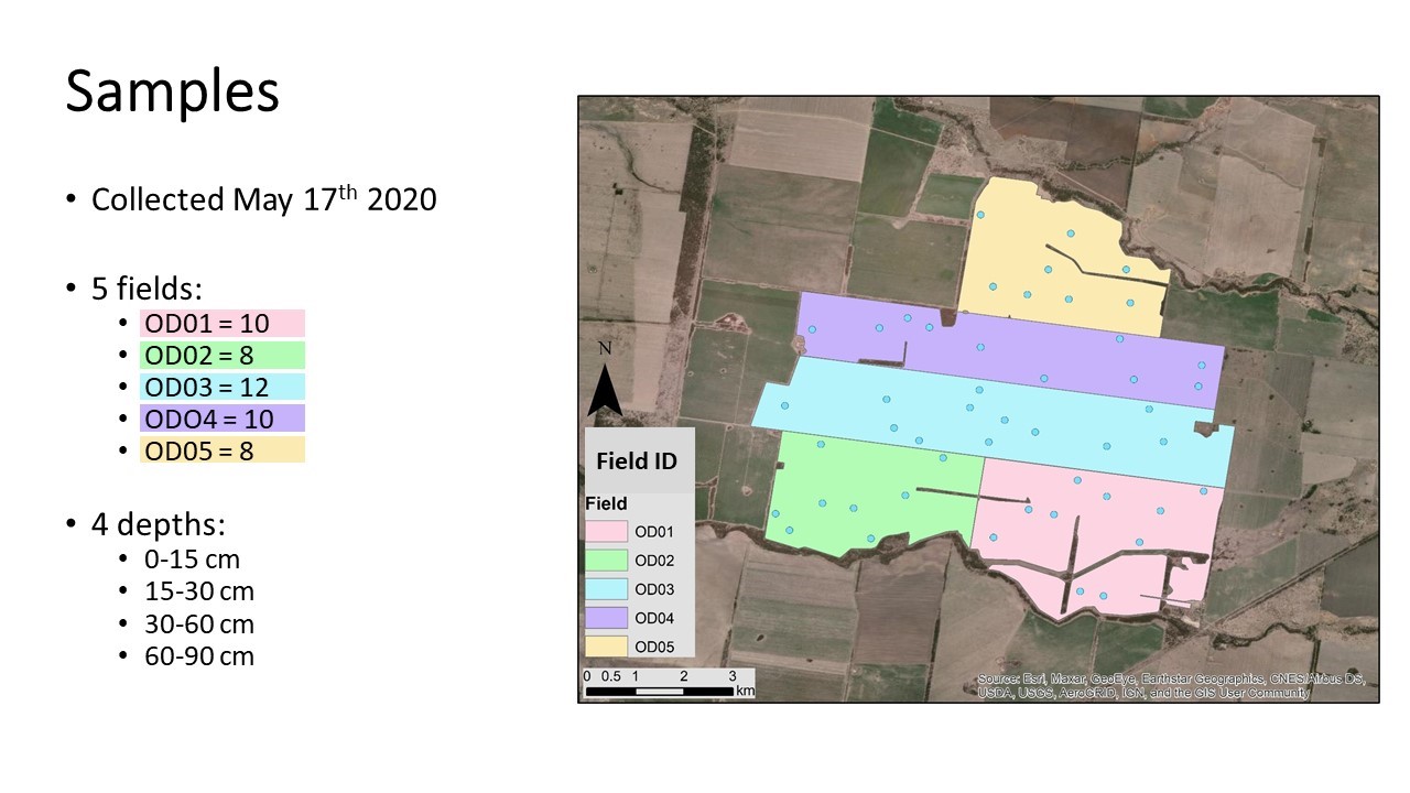
Figure 1. Forty-eight sample locations on the 5000ha test farm.

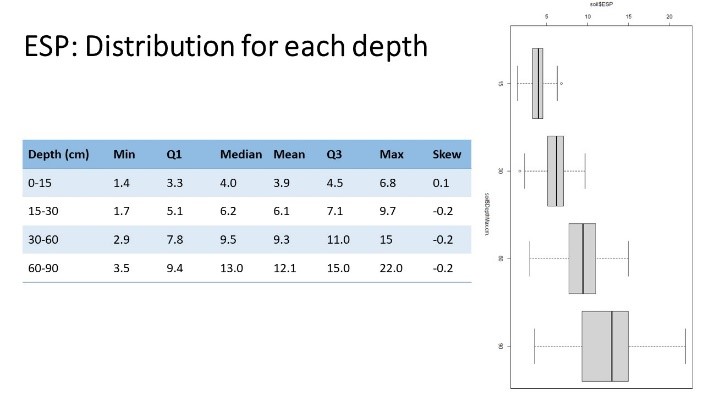
Figure 2. Range of ESP raw data in the 48 samples on the test farm.

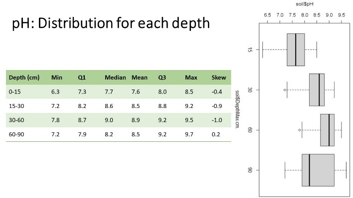
Figure 3. Range of pH raw data in the 48 samples on the test farm.

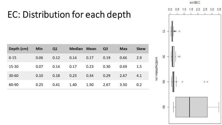
Figure 4. Range of EC raw data in the 48 samples on the test farm.

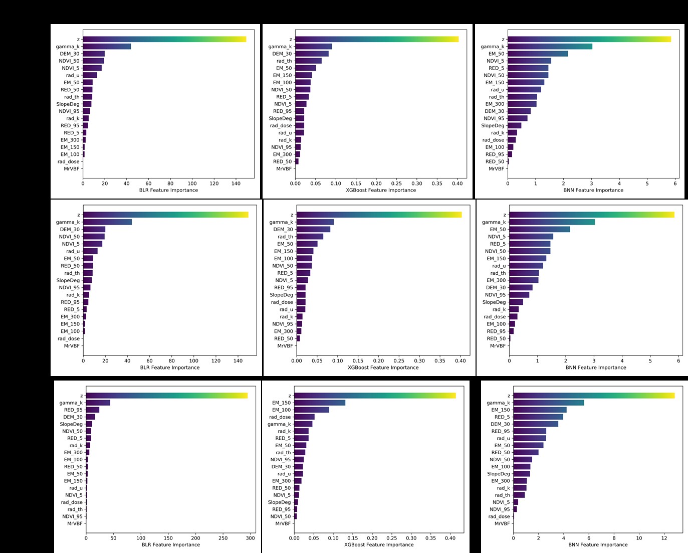
Figure 5. Importance of variables used in the prediction of ESP, pH and EC using 3 different ML models (Bayesian Linear Regression, XG Boost, Bayesian Neural Networks) are ranked. “z” = depth is ranked as number 1 in all models followed predominantly by the “K” band from the gamma radiometric soil survey.The feature importance scales on the x-axis are different because fundamental differences in the modelling approaches impact the method of importance calculation. Ranking and relativity within each model type are the focus.

Table 1. Model fit for ESP data using the different models. The two best methods of the models tested (BNN and BLR) are highlighted. A single model is fitted to describe the variability over the whole profile depth which provides the “mean” model (e.g. BLR) The “+GP” indicates the addition of a Gaussian process on the residuals of the mean model.

Figure 6. Predicted ESP (%) across the farm using BNN plus GP. Profile average ESP and ESP at three different depths down the profile are shown.

Table 2. Model fit for pH data using the different models. The best method of the models tested (BNN) is highlighted. A single model is fitted to describe variability over the whole profile depth which provides the “mean” model (e.g. BLR) The “+GP” indicates the addition of a Gaussian process on the residuals of the mean model.

Figure 7. Predicted pH across the farm using BNN plus GP. Profile average pH and pH at three different depths down the profile are shown.

Figure 8. Predicted EC (mS/cm) across the farm using BNN plus GP. Profile average EC and EC at three different depths down the profile are shown.

Area/volume predictions versus point predictions

In Figure 9a, the ESP is predicted at 30cm depth at the specific points on the whole farm grid. This is an estimate of what the value should be right at each point. In Figure 9b the values represent the average in a 50m x 50m x 0.1m block centred around each point on the whole-farm grid. The standard deviation is reduced by nearly 50% which reduces the uncertainty in the predictions by the same amount.

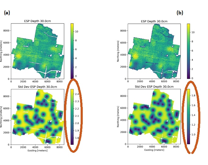
Figure 9. Predicted ESP using BNN plus GP. (a) point predictions and associated standard deviation (Std Dev), and (b) block predictions and associated reduction in Std Dev.

Moving forward

• The BNN and BLR methods will be moved forward to test on more cropping farms to get better information on model performance in different areas and also to test if a reasonable ‘general’ model can be built from data from numerous farms.
• Freely available soil data will be processed to build a cropping-only subset, which will be further subset into regional soil types in order to test for improved value to the prediction process.
• Targeted independent soil sampling to test the maps produced will be undertaken.

Soil water nowcasting for dryland cropping in Australia

This project is a partnership between GRDC, USYD, CSIRO, University of Southern Queensland (USQ) and the BOM. It aims to deliver a scientific framework to nowcast plant available water (PAW). Nowcasting refers to predicting the current state of an attribute of interest. The approach here will be based on digital data but will be agnostic to the type of soil water data streams. It will extract the best features of all in terms of accuracy and spatial and temporal resolution to provide improved PAW predictions using scale-able, modular modelling frameworks that can be operationalised into new analytic products by commercial third-parties. The agnostic nature of the approach means that it should be able to accommodate the next generations of sensors, remote sensing platforms and water balance modelling approaches. The project will test, develop and refine data-driven, data assimilation, soil water balance modelling and ensemble-based approaches, i.e., different analytical frameworks to prediction PAW using the combined expertise of the five different research organisations and strong collaborations with grower networks and industry, including the Society for Precision Agriculture in Australia.

Summary of early results

Due to the declining cost of soil moisture probes, there is an increasing proliferation of soil moisture probe networks across Australia operated by grower groups, universities and state agencies. Many of these offer real-time and publicly available soil water measurements. However, it is unknown whether the networks represent the full range of conditions such as farming systems, terrain, soil, and weather that control the spatial and temporal variability of soil moisture. Therefore, the project's first objective was to assess how representative the current publicly available soil probe networks are of Australia's entire grain cropping region. If they have sufficient coverage and could be calibrated in some way, they could be used in a machine learning model to predict soil moisture or uses to calibrate water balance models.

In addition, a workflow to apply our water balance model for any location in Australia has been developed to provide daily predictions at a 90m resolution for multiple depths in the soil profile. This model will be improved on over the project.

Identification of gaps in current soil moisture probe networks

A digital data cube at a 1km resolution was created for the whole of Australia based on the following data sources which were chosen to represent soil moisture dynamics, focusing on the concepts of soil water storage, soil water use, water flow and the soil properties that influence these processes: (i) soil as represented by the Soil Landscape Grid of Australia; (ii) weather as represented by BOM rainfall and temperature surfaces; (iii) vegetation as represented by Landsat imagery; and, (iv) terrain as represented by elevation, slope and slope-aspect. Table 3 documents the 33 data layers used.

The locations of 371 soil moisture probes installed across grain cropping regions that were accessible to the CSIRO were used to represent the available soil moisture probe network (Figure 10). At these locations, the information from the digital data cube of Australia (33 layers) was extracted to describe the extent of variation in these properties across the soil moisture probe network. The idea being to use a ML technique to compare the extent of variability represented across the probe network to the extent of variability across Australia and the grain cropping regions.

The process used to tackle this issue is based on work done by Meyer and Pebesma (2020). This method delineates the area of applicability (AOA) of a derived model based on a dissimilarity index (DI). The AOA is the area in a multidimensional predictor data space (in this instance the Australia wide data cube of 33 layers) where reliable predictions from a machine learning model made from a training data set (the data extracted at the moisture probe network locations) can be made based on the same input parameters. The DI is based on calculating the distance in the multidimensional data space between data outside the training data to the data used in the training model.

Table 3. Covariates to describe the characteristics of the study area. Seasonally averaged means that there are four different values for the relevant property.

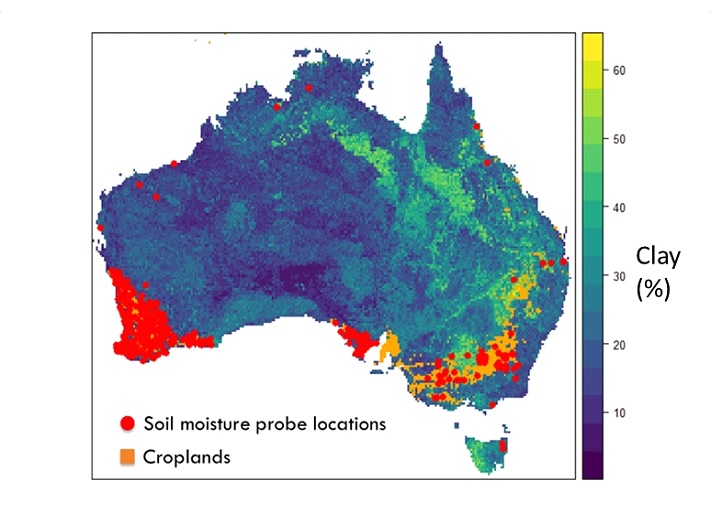
Figure 10. Current soil moisture probe locations overlaying cropland and topsoil clay maps.

The method was implemented using the 'AOA' function from the 'CAST' R package (Meyer and Pebesma, 2020) that uses a Random Forest approach to build the training model using the multidimensional input (probe location data), calculates the DI as comparison with the whole data set (Australia-wide data set) and determines the area of applicability.

Reliable predictions are defined as predictions that can be made with an error that is, on average, comparable to the cross-validation error of the model computed using the training data. This concept is embedded in the use of DI where, if the result of the comparison between a new prediction location and the training model parameters is 0, then the new data point is identical in its values of predictors to the values of the training data set predictors. In this case we can believe our model can be used to predict at the new location. If the value of DI is equal to, or greater than 1, the difference between the new data point and the training model parameters is equal to or larger than the average dissimilarity in the data in the training data set. At this point the prediction error using the model at the new point would be equal or greater than the cross-validation error of the original model, and therefore the point is not suitable for application of the model. A maximum threshold DI value of 0.95 was set to define the AOA in this work.

Figure 11 shows the dissimilarity index calculated for the whole of Australia and Figure 12 shows the AOA for Australia based on the current soil moisture probe networks. As expected, much of Central and Northern Australia sits outside the AOA. The east coast also sits outside the AOA. Figure 13 shows the grain cropping regions overlain on the AOA map.

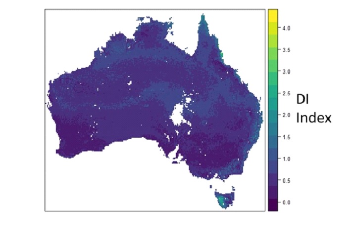
Figure 11. Map of dissimilarity Index: lower values show the minimum distance to training data in the multidimensional predictor space. Areas where there is no data are water bodies.

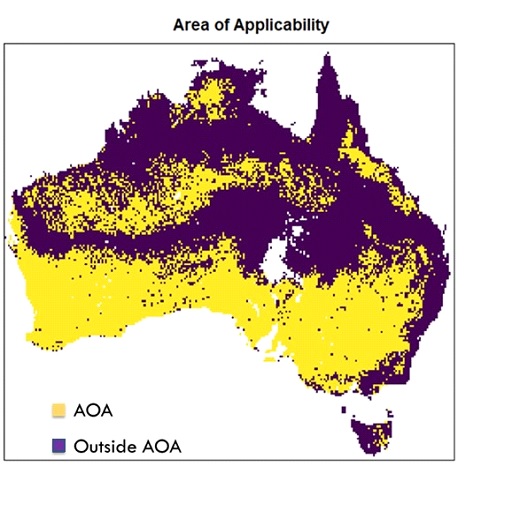
Figure 12. Area of Applicability (AOA) for the model built using the soil moisture probe network data.

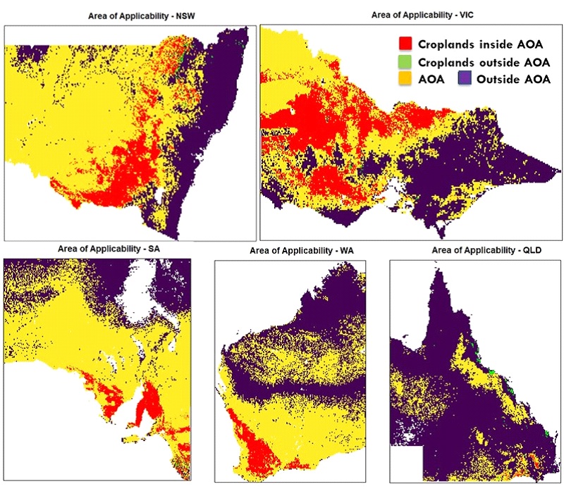
Figure 13. Croplands overlain on the Area of Applicability map.

Table 4. Percentage of cropland covered by the AOA calculated for individual Australian states.

Future work will explore the use of state land use mapping products which have better spatial resolution and apply this approach at a finer resolution (90 m) as compared to the current approach which was performed at 1km.

A prototype of the PAW product

The first series of prototype soil moisture products has been launched on an R Shiny platform, which uses the water balance model introduced by Wimalathunge and Bishop (2019). The predictions are at 90m for multiple depths in the soil profile. Growers, consultants and other industry representatives will be invited to provide feedback on the prototype PAW products via the R Shiny Platform as the project develops. The following links present the prototype PAW product for a few time points at some test locations in NSW. The 1st link presents results for two of USYD’s university farms (Nowley/Llara). The 2nd link is for the Muttama Creek catchment near Cootamundra in southern NSW.  Figure 14 provides an example of a soil water estimate for the USYD Nowley property at a 90m resolution for 30-100 cm.

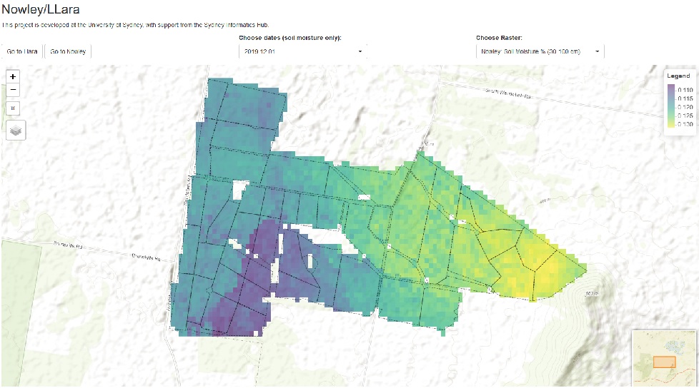
Figure 14. PAW estimates for the USYD property, ‘Nowley’.

The number of locations will be expanded over the life of the project. Growers with an interest in providing feedback on the PAW products which can be applied on their farms should contact thomas.bishop@sydney.edu.au.

Moving forward

• Downscaling of MODIS ET is being undertaken to reduce the resolution of models and therefore predictions to below 1km.
• A process to use the data and models to ‘semi-calibrate’ soil moisture probes is being developed.
• Improvements are being made to the water balance model and we are comparing prediction quality via the use of different precipitation and ET products.
• Field measurement of soil moisture will be collected using CSIRO’s mobile cosmic-ray probe platform (CosmOz Rover) to measure soil moisture in real-time on-the-go and validate our predictions

Conclusions

Future work will consider combining outputs from both projects so that the depth to constraint maps can be used to identify what soil moisture is in the unconstrained part of the soil profile. It is this accessible soil moisture that should be used to guide yield potential estimates and management decisions. Finally, while the quality of our predictions for depth to constraint or soil moisture with field observations can be tested the true test is whether these data products can improve management decisions. This can be achieved with on-farm experimentation which is possible with variable-rate technology.

References

Meyer, H. and Pebesma, E., 2020. Predicting into unknown space? Estimating the area of applicability of spatial prediction models.

Wimalathunge, N. and Bishop, T., 2019. A space-time observation system for soil moisture in agricultural landscapes. Geoderma, 344, pp.1-13.

Acknowledgements

The research undertaken as part of this project is made possible by the significant contributions of growers through both trial cooperation and the support of the GRDC, the authors would like to thank them for their continued support.

Contact details

Tom Bishop
Precision Agriculture Laboratory, Sydney Institute of Agriculture, The University of Sydney
Biomedical Building, Australian Technology Park, Eveleigh NSW 2015
02 8627 1132
thomas.bishop@sydney.edu.au