Can assimilating remote and proximal sensing observations into the Agricultural Production Simulator crop model improve wheat yield prediction accuracy without calibrating against observed yield
Author: Ian Marang (The University of Sydney) | Date: 24 Feb 2022
Take home messages
- Mid-season predictions of end season crop production can be achieved by using potential yield with only a limited set of field condition observations collected remotely.
- Assimilating mid-season remote and proximal sensing observations can improve APSIM model predictions of wheat yield.
Abstract
There is increasing pressure on agriculture to deliver the food and fibre production necessary to meet the rising demand of a growing population while reducing inputs and impacts on the environment. To meet these challenges, growers need more accurate estimates of mid-season crop condition and potential yield under variable future growing circumstances. Assimilating mid-season remote sensing observations of crop status into process-based crop models can be a useful tool to provide these estimates. This project tests if assimilating remote and proximal sensing observations into the APSIM crop model can improve wheat yield prediction accuracy without calibrating against observed yield. This is achieved by using a sensitivity analysis to map the weighting from the errors between crop condition simulations and observations with the model parameters’ individual impact on outputs and taking the mean of an ensemble of predictions.
Results indicate remote sensing has strong potential for sampling crop status with high spatial, spectral and temporal resolution, as seen with accurate protein concentration estimation (r2 of 0.88 in 2020) and strong yield prediction (r2 of 0.64 in 2019). There are substantial confounding aspects to collecting and interpreting remote sensing data, however, due to the high dependency of plant condition on factors outside the scope of observation, including interannual and intraseasonal climate and phenology variation, biotic and abiotic stresses, and viewing geometry, amongst others. These factors may be behind the lower accuracy seen in comparisons across the two years’ experiments, such as protein concentration in 2019 (r2 of 0.29) and yield prediction in 2020 (r2 of 0.32).
Crop models are able to simulate the processes that remote sensing or statistical models cannot, but to do this they need effective parameterisation and calibration. ‘Sobol’ sensitivity analysis was run on the APSIM crop model using five different block sizes with three perturbed model physics ensemble members. This generated a total of 576 000 simulations which were used to identify the relative influence of 23 parameters after their ‘Sobol’ confidence intervals had stabilised and reached approximately 0.05 on average. After 96 000 runs, each ensemble had stabilised and indices were reported, showing APSIM constants controlling radiation use efficiency and soil water extraction were the most influential. Cultivar parameters were the least influential across all the output variables and block sizes tested. The main effect indices were then averaged across the season and used in the crop modelling data assimilation framework. Data assimilation is a technique to check model performance against observed conditions and update the model for improved accuracy.
For use in the data assimilation framework, a group of model simulations (i.e., an ensemble) was built with small variations in the key factors that impact crop modelling prediction uncertainty: management action (four or six nitrogen fertiliser rates), observations (11 sets of weather), parameterisation (three levels of soil condition) and model structure (three examples of altered physics). These ensemble members were run over 15 iterations of the 2019 and 2020 seasons using calibrated and uncalibrated parameters, with their parameters modified between iterations using the relative errors in their predictions scaled by the sensitivity indices. Error weighting was derived from comparing predicted height growth, water extraction and yield against height growth from RGB photogrammetry, water extraction from soil moisture probes and potential yield from a statistical model. The mean of each ensemble was tested against observed yield for the year as well as APSIM performance without data assimilation. Results indicate there is strong potential for this approach, with average improvements between 7-12% of observed yield in all tests. The data assimilation framework delivered substantial improvements over both the standard run and a simple statistical model built using 12 seasons of yield data and weather from a nearby site. This project shows assimilating mid-season remote and proximal sensing observations can improve APSIM model predictions of wheat yield.
Background
Food security is an increasing concern with the rising demand from a global population projected to reach 9 billion by 2050 [1]. Exacerbating this are the large-scale impacts to growing conditions, both current and prospective, of a changing climate [2], [3]. There are a number of efforts to address the challenge of increasing production of food and fibre, including plant breeding [4], [5], more efficient and sustainable farm production methods [6], [7] and building a better understanding of food production through crop models [8]–[11]. Remote sensing is a useful tool to infer crop status at scale, but is less effective at direct numerical evaluation and prediction [12]–[14]. Crop growth models, in comparison, can be robust at prediction but are fundamentally abstract constructs that cannot accurately replicate all processes that contribute to plant production [15]. By assimilating observations of a crop mid-season, the missing aspects of these models, such as pests or disease impacts can be adjusted for and so generate more plausible estimates of plant condition and production [16].
Process-based models can be used for investigating regional or global projected changes on a macro scale, but also informing grower management action on a local level [17]. There is a wide assortment of models being used, however, most are either for use in very specific fields (for example, studies of soil organic matter processes, such as DayCent, see review by Brilli et al. 2017), or are no longer being developed and supported (such as CENTURY, see review by Jin et al. 2018). Most are based on a daily time step and involve incrementing plant biophysical condition as a function of weather forcing (for example, rainfall amount, maximum and minimum temperature), soil nutrients and moisture available for plant extraction, and selected management actions, with limits and coefficients given by genetic parameters which are related to a sown cultivar [20], [21].
Simulating soil dynamics and climate extremes are areas where models require further development [1], [18]. Additionally, most models poorly simulate grain protein content and quality parameters, possibly due to incorrect N mobilisation estimates and an emphasis on yield over other outputs [17], [22]. However, many models manage to estimate yield effectively by balancing intra-seasonal modelling errors and structural inconsistency (for example, where errors in one part of the model can be balanced out by others in different parts), suggesting model efficacy should not be judged based on a single variable [17]. One approach to overcome these modelling challenges, is to use an ensemble of models, whereby multiple instances of the same model, or multiple instances of different models are run with the same or similar forcing data and simulate the same crop [1]. This has seen increasing usage, especially in the climate change impact assessment community where ensembles of twenty or thirty models combined are common [17], [23], [24]. However, ensembles as small as two or three models have been reported to improve estimation accuracy considerably [25]. In several previous studies, the median or mean of all ensemble members had superior accuracy over any of the individual models. That’s possibly because the ensemble balanced out the individual model design errors or had access to all the datasets used to calibrate the individual models by proxy, and therefore better sampled the variability of crop growth under study [1], [17], [23], [26]–[28]. Ensembles may also provide a direct estimate of the uncertainty of the prediction [29].
The objectives of this study were to test if remotely sensed crop height and soil moisture observations can be combined with a statistical model’s estimate of yield from rainfall and assimilated into a process-based crop growth model, the Agricultural Production SIMulator (APSIM) to improve yield prediction. At the time this research began there were limited previous studies on assimilating remote sensing observation with APSIM. The authors coupled a radiative transfer model with APSIM outputs for use with satellite optical reflectance data to predict biomass in maize. They found that data assimilation was successful at improving the modelled biomass in most cases [42]. Another used spatial variation across a field to drive yield spatial variability [43]. In contrast, this study assimilates the predictions of a statistical model and direct observations from a UAV platform and soil moisture probes into APSIM to improve predictions of wheat yield.
Methodology
There were three main components to this project:
- Two field trials of wheat were held (one each in 2019 and 2020) to collect remote and proximal sensing observations for assimilating into the crop model (Figure 1). The ability of remote sensing to quantify the observed crop condition and production was tested using actual and combined measures of reflectance (vegetation indices).
- A sensitivity analysis was run to map the influence of twenty-three selected parameters on the crop model’s output. This section identifies the key levers of model performance on the output matching the observations from the field trials.
- A data assimilation framework was built to run the APSIM crop model iteratively over a large group (396 in 2019 and 594 in 2020) of models, each containing different combinations of estimates of weather, soil condition, model structure and fertiliser applications. The average of the group of model predictions before and after data assimilation were compared to see if in-season crop simulation and yield prediction accuracy were improved.
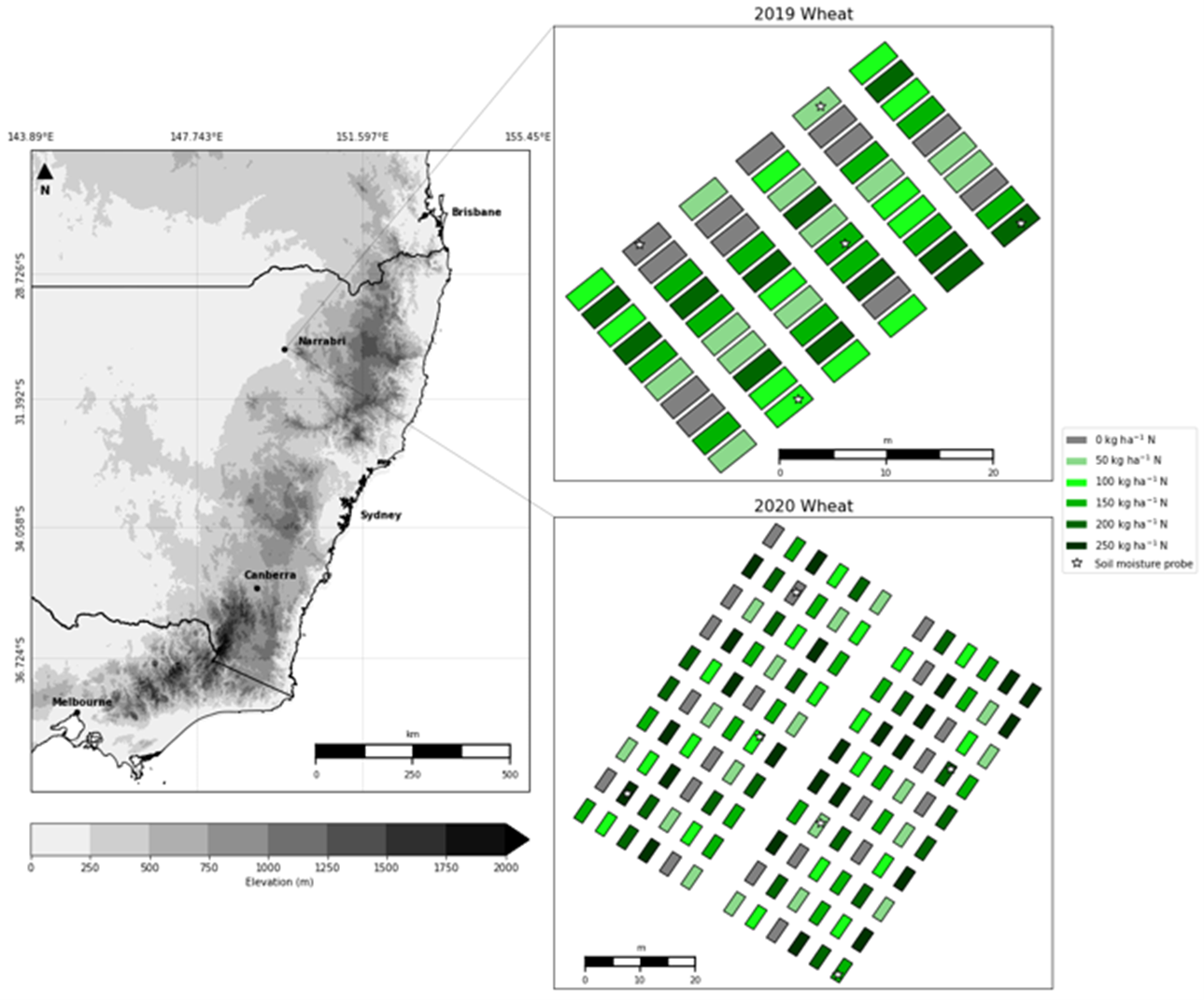
Figure 1. Regional map showing locations of 2019 and 2020 wheat experiments.
Four tests were run, with the APSIM DA framework (Figure 2) using calibrated and default genetic and soil parameters for 2019 and 2020 for the first run, with potential modifications in subsequent runs in response to the errors during assimilation. The iteration (i) determined when the test was complete and if the conversion factor applied to model parameters should be inverted if errors had increased.
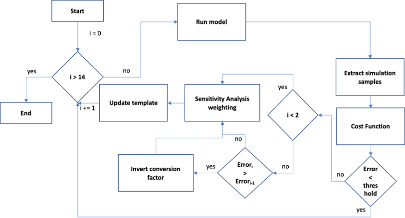
Figure 2. Data assimilation framework conceptual flowchart.
Results
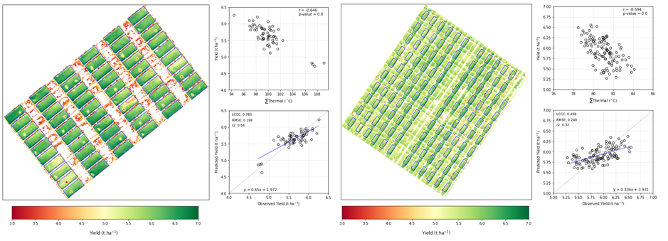
Remote sensing showed strong relationships between reflectance and thermal imagery and observed crop characteristics or end season production, but with very limited consistency between years. For example, 2019 yield prediction was strong using thermal (R2 of 0.64), but 2020 yield prediction using thermal was substantially weaker (R2 of 0.32) (Figure 3).
Figure 3. Sum of thermal remote sensing over four sample dates in 2019 (left) and 2020 (right) predictions of yield, note predictions <3t/ha were made null.
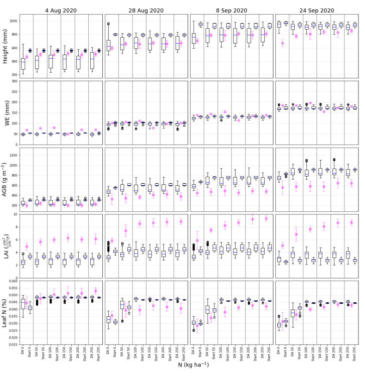
After data assimilation, crop condition predictions accuracy saw improvement in height estimation and above ground biomass but not so leaf area index, which had a very mixed outcome. Soil moisture and leaf N % were already very close to the observations before data assimilation (Figure 4).
Figure 4. Crop condition performance of the standard and DA APSIM model runs for the calibrated test in 2020 for the six tested N levels and four sample dates. ‘Start’ in the plot refers to the model runs in only the first iteration using only the default model physics. Height is plant height; WE is water extraction, AGB is aboveground biomass; LAI is leaf area index and leaf N % is leaf nitrogen concentration. Average observed values are shown as circles with errors bars for the standard deviation. Note the water extraction was measured at a single point and so has no standard deviation.
Yield prediction improved in all four tests, more so in 2019 (Figure 5) as the water use efficiency model’s error signal was much stronger in 2019 than in 2020 (Figure 6) due to lower in-season rainfall leading to a lower potential yield threshold.
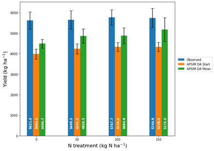
Figure 5. Yield predictions of APSIM before (using only the default physics; ‘DA Start’) and after data assimilation (‘DA Mean’) compared with average observed values in 2019. Error bars show the standard deviation and the average values are printed at the base of the columns.
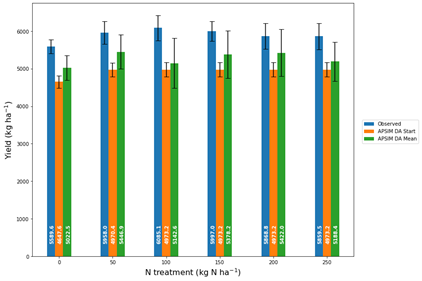
Figure 6. Yield predictions of APSIM before (using only the default physics; ‘DA Start’) and after data assimilation (‘DA Mean’) compared with average observed values in 2020. Error bars show the standard deviation and the average values are printed at the base of the columns.
Conclusion
This project consisted of two field trials of wheat, with remote sensing and soil moisture observations, complemented by in-season crop condition sampling. A sensitivity analysis was performed on the APSIM crop model to find the relative influence of each of the 23 parameters chosen from a review of the relevant literature. The sensitivity analysis results were then applied as scaling to the error weighting from comparing potential yields, and remote sensing and soil moisture observations with model predictions in a multi-model ensemble Data Assimilation (DA) framework to test if prediction fit could be improved.
The ensemble mean yield prediction after DA outperformed the standard APSIM prediction using the default physics, on average, by between 7-12% for all four tests, although, more so for 2019 than 2020. Uncalibrated tests showed larger improvements, although this was from a much lower baseline accuracy. The range of variation added through ensemble factors stretched the range of potential model states, and therefore captured more of the natural range of outcomes seen in the field. The scaling from the sensitivity analysis may have reduced the impact of parameter interactions by minimising the impact of parameters that were less influential and maximising those with higher influence. Further, the parameter weighting provided by assimilating errors in the fit between observed and predicted state variables (i.e., height growth, water extraction and potential yield) guided the model towards more realistic estimates of crop status.
While the main focus of this project was yield prediction accuracy improvement, for farmers and agronomists in-season crop condition is important for delivering better outcomes at the end of the season, as well as building confidence that the model is getting the ‘right answer for the right reason’. The DA ensemble’s iterative adjustment over the modelling runs resulted in mean crop condition during the season being improved over the standard in most output variables on most dates. Several key dates showed large improvements in accuracy, such as the 28 August and 8 September having near identical simulated and observed mean heights in the calibrated test in 2020, however, all dates showed improvement in height estimation. The improvements for other variables were not uniform, however, as shown by the predictions of LAI for the first through to the third sample date in 2020 being generally less accurate after the DA framework than for standard APSIM. The results for 2019 were similar, however, with slightly better results in LAI and slightly less successful height adjustment. APSIM predictions were generally strong for both the standard and DA ensemble in leaf N and water extraction.
In order to test the generality of the approach and whether a mid-season application of the DA ensemble framework was possible, neither during calibration nor the model runs did the DA framework reference actual observed yield from either year. Instead, the predicted yield during the runs were tested against the French and Schultz Water Use Efficiency (WUE) model, as a proxy for potential yield. After the data assimilation, the results were tested against observed yield (Figures 5 & 6). For the 2019 calibrated test, this was successful in improving the yield predictions. The 2020 calibrated test was predicting yield greater than the WUE model from the first iteration, due to a lower threshold from less rain having been received in-season, however, yield predictions continued to improve due to the height and water extraction assimilation. This highlights the practical application of this research for farm managers and advisers: mid-season predictions of end season crop production can be achieved by using potential yield with only a limited set of field condition observations collected remotely.
Useful resources or References
[1] A. Maiorano et al., “Crop model improvement reduces the uncertainty of the response to temperature of multi-model ensembles,” Field Crops Research, vol. 202, pp. 5–20, 2017, doi: 10.1016/j.fcr.2016.05.001.
[2] A. Iglesias et al., “Adaptation to Climate Change in the Agricultural Sector,” 2007. doi: 10.1590/s1809-98232013000400007.
[3] Intergovernmental Panel on Climate Change, “Summary for Policymakers. Climate Change 2021: The Physical Science Basis.,” Cambridge University Press, 2021.
[4] M. Reynolds et al., “Achieving yield gains in wheat,” Plant, Cell and Environment, vol. 35, no. 10, pp. 1799–1823, 2012, doi: 10.1111/j.1365-3040.2012.02588.x.
[5] J. Tack, A. Barkley, and L. L. Nalley, “Effect of warming temperatures on US wheat yields,” Proceedings of the National Academy of Sciences, vol. 112, no. 22, pp. 6931–6936, 2015, doi: 10.1073/pnas.1415181112.
[6] M. G. Lampridi, C. G. Sørensen, and D. Bochtis, “Agricultural sustainability: A review of concepts and methods,” Sustainability (Switzerland), vol. 11, no. 18, 2019, doi: 10.3390/su11185120.
[7] S. F. Bender and M. G. A. van der Heijden, “Soil biota enhance agricultural sustainability by improving crop yield, nutrient uptake and reducing nitrogen leaching losses,” Journal of Applied Ecology, vol. 52, no. 1, pp. 228–239, 2015, doi: 10.1111/1365-2664.12351.
[8] J. W. White, G. Hoogenboom, B. A. Kimball, and G. W. Wall, “Methodologies for simulating impacts of climate change on crop production,” Field Crops Research, vol. 124, no. 3, pp. 357–368, 2011, doi: 10.1016/j.fcr.2011.07.001.
[9] J. W. Jones et al., “Toward a new generation of agricultural system data, models, and knowledge products: State of agricultural systems science,” Agricultural Systems, vol. 155, pp. 269–288, 2017, doi: 10.1016/j.agsy.2016.09.021.
[10] B. A. Keating et al., “An overview of APSIM, a model designed for farming systems simulation,” European Journal of Agronomy, vol. 18, no. 3–4, pp. 267–288, 2003, doi: 10.1016/S1161-0301(02)00108-9.
[11] C. Rosenzweig et al., “The Agricultural Model Intercomparison and Improvement Project (AgMIP): Protocols and pilot studies,” Agricultural and Forest Meteorology, vol. 170, pp. 166–182, 2013, doi: 10.1016/j.agrformet.2012.09.011.
[12] M. Weiss, F. Jacob, and G. Duveiller, “Remote sensing for agricultural applications: A meta-review,” Remote Sensing of Environment, vol. 236, no. November 2019, p. 111402, 2020, doi: 10.1016/j.rse.2019.111402.
[13] D. A. Kasampalis, T. K. Alexandridis, C. Deva, A. Challinor, D. Moshou, and G. Zalidis, “Contribution of remote sensing on crop models: A review,” Journal of Imaging, vol. 4, no. 4, 2018, doi: 10.3390/jimaging4040052.
[14] R. Main, M. A. Cho, R. Mathieu, M. M. O’Kennedy, A. Ramoelo, and S. Koch, “An investigation into robust spectral indices for leaf chlorophyll estimation,” ISPRS Journal of Photogrammetry and Remote Sensing, vol. 66, no. 6, pp. 751–761, 2011, doi: 10.1016/j.isprsjprs.2011.08.001.
[15] J. W. Jones et al., “Brief history of agricultural systems modeling,” Agricultural Systems, vol. 155, pp. 240–254, 2017, doi: 10.1016/j.agsy.2016.05.014.
[16] W. A. Dorigo, R. Zurita-Milla, A. J. W. de Wit, J. Brazile, R. Singh, and M. E. Schaepman, “A review on reflective remote sensing and data assimilation techniques for enhanced agroecosystem modeling,” International Journal of Applied Earth Observation and Geoinformation, vol. 9, no. 2, pp. 165–193, 2007, doi: 10.1016/j.jag.2006.05.003.
[17] P. Martre et al., “Multimodel ensembles of wheat growth: Many models are better than one,” Global Change Biology, vol. 21, no. 2, pp. 911–925, 2015, doi: 10.1111/gcb.12768.
[18] L. Brilli et al., “Review and analysis of strengths and weaknesses of agro-ecosystem models for simulating C and N fluxes,” Science of the Total Environment, vol. 598, no. March, pp. 445–470, 2017, doi: 10.1016/j.scitotenv.2017.03.208.
[19] X. Jin et al., “A review of data assimilation of remote sensing and crop models,” European Journal of Agronomy, vol. 92, no. May 2017, pp. 141–152, 2018, doi: 10.1016/j.eja.2017.11.002.
[20] D. B. Lobell and S. Asseng, “Comparing estimates of climate change impacts from process- based and statistical crop models,” Environmental Research Letters, vol. 12, no. 015001, pp. 1–12, 2017, doi: 10.1088/1748-9326/015001.
[21] M. Ahmed et al., “Calibration and validation of APSIM-Wheat and CERES-Wheat for spring wheat under rainfed conditions: Models evaluation and application,” Computers and Electronics in Agriculture, vol. 123, pp. 384–401, 2016, doi: 10.1016/j.compag.2016.03.015.
[22] J. G. Nuttall, G. J. O’Leary, J. F. Panozzo, C. K. Walker, K. M. Barlow, and G. J. Fitzgerald, “Models of grain quality in wheat—A review,” Field Crops Research, vol. 202, pp. 136–145, 2017, doi: 10.1016/j.fcr.2015.12.011.
[23] S. Asseng et al., “Rising temperatures reduce global wheat production,” Nature Climate Change, vol. 5, no. 2, pp. 143–147, 2015, doi: 10.1038/nclimate2470.
[24] B. Liu et al., “Similar estimates of temperature impacts on global wheat yield by three independent methods,” Nature Climate Change, vol. 6, no. 12, pp. 1130–1136, 2016, doi: 10.1038/nclimate3115.
[25] A. C. Ruane et al., “Multi-wheat-model ensemble responses to interannual climate variability,” Environmental Modelling and Software, vol. 81, pp. 86–101, 2016, doi: 10.1016/j.envsoft.2016.03.008.
[26] X. Yin et al., “Multi-model uncertainty analysis in predicting grain N for crop rotations in Europe,” European Journal of Agronomy, vol. 84, pp. 152–165, 2017, doi: 10.1016/j.eja.2016.12.009.
[27] R. P. Rötter et al., “Simulation of spring barley yield in different climatic zones of Northern and Central Europe: A comparison of nine crop models,” Field Crops Research, vol. 133, pp. 23–36, 2012, doi: 10.1016/j.fcr.2012.03.016.
[28] I. Iocola et al., “Can conservation tillage mitigate climate change impacts in Mediterranean cereal systems? A soil organic carbon assessment using long term experiments,” European Journal of Agronomy, vol. 90, no. July, pp. 96–107, 2017, doi: 10.1016/j.eja.2017.07.011.
[29] J. Verrelst et al., “Optical remote sensing and the retrieval of terrestrial vegetation bio-geophysical properties - A review,” ISPRS Journal of Photogrammetry and Remote Sensing, vol. 108, pp. 273–290, 2015, doi: 10.1016/j.isprsjprs.2015.05.005.
[30] J. Huang et al., “Assimilation of remote sensing into crop growth models: Current status and perspectives,” Agricultural and Forest Meteorology, vol. 276–277, no. May, p. 107609, 2019, doi: 10.1016/j.agrformet.2019.06.008.
[31] H. Moradkhani, “Hydrologic remote sensing and land surface data assimilation,” Sensors, vol. 8, no. 5, pp. 2986–3004, 2008, doi: 10.3390/s8052986.
[32] C. Montzka, H. Moradkhani, L. Weihermüller, H. J. H. Franssen, M. Canty, and H. Vereecken, “Hydraulic parameter estimation by remotely-sensed top soil moisture observations with the particle filter,” Journal of Hydrology, vol. 399, no. 3–4, pp. 410–421, 2011, doi: 10.1016/j.jhydrol.2011.01.020.
[33] R. H. Reichle, D. B. McLaughlin, and D. Entekhabi, “Hydrologic Data Assimilation with the Ensemble Kalman Filter,” Monthly Weather Review, vol. 130, no. 1, pp. 103–114, 2002, doi: 10.1175/1520-0493(2002)130<0103:hdawte>2.0.co;2.
[34] T. Hilker et al., “Data assimilation of photosynthetic light-use efficiency using multi-angular satellite data: II Model implementation and validation,” Remote Sensing of Environment, vol. 121, pp. 287–300, 2012, doi: 10.1016/j.rse.2012.02.008.
[35] G. S. Nearing, W. T. Crow, K. R. Thorp, M. S. Moran, R. H. Reichle, and H. V. Gupta, “Assimilating remote sensing observations of leaf area index and soil moisture for wheat yield estimates: An observing system simulation experiment,” Water Resources Research, vol. 48, no. 5, pp. 1–13, 2012, doi: 10.1029/2011WR011420.
[36] W. T. Crow and E. F. Wood, “The assimilation of remotely sensed soil brightness temperature imagery into a land surface model using Ensemble Kalman filtering: A case study based on ESTAR measurements during SGP97,” Advances in Water Resources, vol. 26, no. 2, pp. 137–149, 2003, doi: 10.1016/S0309-1708(02)00088-X.
[37] A. De Wit, G. Duveiller, and P. Defourny, “Estimating regional winter wheat yield with WOFOST through the assimilation of green area index retrieved from MODIS observations,” Agricultural and Forest Meteorology, vol. 164, pp. 39–52, 2012, doi: 10.1016/j.agrformet.2012.04.011.
[38] R. Li et al., “Assimilation of remote sensing and crop model for LAI estimation based on ensemble kaiman filter,” Agricultural Sciences in China, vol. 10, no. 10, pp. 1595–1602, 2011, doi: 10.1016/S1671-2927(11)60156-9.
[39] S. Moulin, A. Bondeau, and R. Delecolle, “Combining agricultural crop models and satellite observations: From field to regional scales,” International Journal of Remote Sensing, vol. 19, no. 6, pp. 1021–1036, 1998, doi: 10.1080/014311698215586.
[40] X. Mo, S. Liu, Z. Lin, Y. Xu, Y. Xiang, and T. R. McVicar, “Prediction of crop yield, water consumption and water use efficiency with a SVAT-crop growth model using remotely sensed data on the North China Plain,” Ecological Modelling, vol. 183, no. 2–3, pp. 301–322, 2005, doi: 10.1016/j.ecolmodel.2004.07.032.
[41] G. Evensen, Data Assimilation: The Ensemble Kalman Filter, 2nd Editio. Springer Berlin Heidelberg, 2009.
[42] M. Machwitz et al., “Enhanced biomass prediction by assimilating satellite data into a crop growth model,” Environmental Modelling and Software, vol. 62, pp. 437–453, 2014, doi: 10.1016/j.envsoft.2014.08.010.
[43] Y. Zhang, J. P. Walker, V. R. N. Pauwels, and Y. Sadeh, “Assimilation of wheat and soil states into the apsim-wheat crop model: A case study,” Remote Sensing, vol. 14, no. 1, Jan. 2022, doi: 10.3390/rs14010065.
Contact details
Ian Marang
The University of Sydney, Researcher PhD Student
ian.marang@dpi.nsw.gov.au
Was this page helpful?
YOUR FEEDBACK

