The valuation of agricultural assets in Australia
Author: Tim Lane ( Herron Todd White) | Date: 06 Jun 2017
Take home messages
- The valuation of agricultural assets in Australian underpins the agriculture land market for purchasers, sellers (vendors), neighbouring farmers, banking and investment sectors.
- The rigour and accuracy in the valuation role is imperative in this process.
- There are a myriad of methods and approaches used to value agricultural land.
- Valuers often only have limited access to vital information like farm performance data, seasonal conditions, commodity price fluctuations, buyer motivation, and locational advantages or disadvantages. As a consequence, a valuer can find it quite challenging to apply capitalisation rate for investors and give them indicators that are utilised commonly in the corporate investment world.
Introduction
The decision to invest in agricultural land in Australia has traditionally been made without accurate historical knowledge of the financial return available from a particular property. Purchasers base their decisions on direct comparison with sales of other, similar farming properties, coupled with their personal view of what return will be achieved from the property.
Agricultural land is a key asset of a farming operation. As a major asset is subject to a value, it is common for many rural properties/agricultural land to be valued on past sales in local areas/districts. One aspect of the rural valuation market is at times a lack of actual sales on which to determine value, which is unlike residential and commercial property investment that generally has well defined investment criteria and a relatively liquid market.
With many years’ experience as an independent property adviser, a regular question I hear is: ‘What is the expected return from a property relative to the price paid?’ This is a common question throughout the valuation industry, which has been highlighted in more recent times with the increasing international interest in the sector. The combination of recent Free Trade agreements with China, Korea, Japan and the potential of the Trans Pacific Partnership, a falling cost of debt, a rising global population and falling energy costs have created the environment for non-traditional investors to look at the agriculture sector as an attractive investment asset class. These experienced investors expect to look at standard investment indicators like the percentage of net return on capital. Unfortunately however, the rural market has not evolved to be able to provide these type of asset measurements.
This paper will define and consider the current market value methodologies used to value agricultural assets in Australia. It begins by identifying the different approaches within the agricultural industry that a valuer can utilise and defines such methods. The paper will then consider the influences of a sale transaction and how it can affect the price paid for an agricultural property. A number of elements that have a direct influence on the value of a property are:
- the available data about the property performance and that of the agricultural business,
- seasonal conditions, and
- the capitalisation rate along with buyer motivation and locational advantages.
The final section of the paper explores the trends of rural debt in Queensland and the impact of commodity price fluctuations on the value of agricultural land.
For the purposes of this paper, an agricultural asset will be defined as:
The property is on an area of land greater than 50 hectares (ha) and:
- where the assessed gross income from primary production exceeds $30,000 per annum,
- where construction of a dwelling on the property is not permitted, or
- where the property features associated water entitlements/licences or is connected to an irrigation system.
Market value and methodologies
If a property does not make a profit (and therefore no real return in a year) it does not automatically follow that the asset has a nil value. There are many seasonal and other factors which will apply across the Australian rural landscape that influence the return profile in any one year, however these assets will still retain a relative value in the market place.
So why is this the case and what could be developed over time to help provide guidance to an investor regarding likely returns, rather than simply saying that the property can carry 2000 adult equivalent (AE) head of cattle?
The concept of market value originates from legal precedent and dates back to 1907.
Market value is the estimated amount for which a property should exchange on the date of valuation between a willing buyer and a willing seller in an arm’s-length transaction after proper marketing wherein the parties had each acted knowledgeably, prudently, and without compulsion.
The definition arises from the Australian compensation case Spencer v The Commonwealth of Australia (1907), 5 CLR 418 in which Griffiths CJ stated:
Bearing in mind that value implies the existence of a willing buyer as well as of a willing seller, some modification of the rule must be made in order to make it applicable to the case of a piece of land which has any unique value. It may be that the land is fit for many purposes, and will in all probability be soon required for some of them, but there may be no one actually willing at the moment to buy it at any price. Still it does not follow that the land has no value. In my judgment the test of value of land is to be determined, not by inquiring what price a man desiring to sell could actually have obtained for it on a given day, i.e., whether there was in fact on that day a willing buyer, but by inquiring, ‘What would a man desiring to buy the land have had to pay for it on that day to a vendor willing to sell it for a fair price but not desirous to sell?’
The valuer’s role is to interpret why the market has paid a particular level of value for assets by undertaking a correct and proper analysis of the evidence to ‘look behind’ the sale, being conscious not to just accept the sale on face value. From that they can then draw upon their professional opinion to determine the value. Within the agricultural industry some of the methodologies utilised to determine value include:
- Direct comparison approach: This requires the valuer to make adjustments, usually on a subjective basis, around the relative strengths and weaknesses of one property compared to another.
- Summation approach: This requires the valuer to further analyse the sales evidence in order to show separate levels for different land class types, irrigation water entitlements as well as structural improvements including dwellings. This information is then used to apply separate levels to the various components of the property being valued.
- Productivity approach: This approach is commonly used when valuing extensive grazing properties and requires the valuer to analyse the sales evidence to show a rate per unit of livestock able to be carried. This information is then used to determine the value of the property being valued, based on an assessment of its carrying capacity. This approach is also useful when valuing intensive livestock industries such as piggeries or chicken farms. Some standard units of measure are:
- AE – adult equivalent – a 450kg steer or non-lactating cow.
- DSE – dry sheep equivalent – a 45kg wether or non-lactating ewe on a maintenance diet.
- CSU – standard cattle unit – A 600kg steer or cow in a feedlot.
- $/Bird – relates to poultry assessments for meat production.
- Income approach: This approach, which is the common way that commercial buildings are valued, requires an assessment of the likely future net return from a particular property, which is then capitalised at a yield that is determined from analyse of comparable sales. This approach is rarely, if ever, used.
- Discounted cash flow approach: This requires the valuer to model the expected income and net profit from a particular farm and then convert this expected income stream into an acceptable purchase price, based on the expectation of a particular rate of return. The discounted cash flow approach is generally regarded as a check method rather than prime method of valuation, due to the need to make assumptions around yield, commodity prices and operating expenses.
Buyer and seller influences
So what influences come into play when a buyer or seller enters into a sale transaction and how does this effect the price paid?
For the purposes of this discussion I have elected to not get into the technical standards and professional indemnity issues that the valuation industry are required to operate within. This includes the legal precedents of valuers being successfully litigated against when seeking to adopt an income approach for an agricultural assessment. The matters raised in this discussion will focus on the variable aspects of agriculture, and therefore, variable financial performance of the sector.
Available data
One of the key requirements to assess a property on a financial return basis is access to verifiable data. In the majority of cases (regardless of whether bank or owner instructed), the valuer is not provided with copies of the last three to five years’ trading and production figures for the business. At best they will get copies of stock books to understand the stocking densities relative to seasons, maybe a property plan, a summary of capital expenditure in recent periods and some rainfall data. The balance of information relevant to the property’s financial performance is usually anecdotal, for example branding rates, yield from crops, bales per hectare for cotton, etc.
The other aspect of the financial data produced by most accounting firms is that they tend to compress the data to fit a format. A grazing enterprise will normally include a livestock trading account, which shows opening and closing stock, sales and purchases, death and rations which is balanced annually. However the farmer will rarely sell a uniform number of livestock each year. For a multitude of reasons, a much higher or lower number of stock will invariably be sold in some years. For cropping enterprises, the financial statements do not include the area cropped, total yields (measurements of production), nor a value of any unharvested crop or summary of grain being stored on farm in the hope that prices will increase. This means that the basis to draw a verifiable conclusion about the annual financial return from an enterprise is limited.
Even if more detailed financial data were provided to a valuer, the next matter would be the standardisation of this data to reflect a ‘true business’ cost as opposed to what the farmer reflects in the financial statements. Every business owner will manage the expenses within the business differently, and also to their benefit, sometimes these decisions around expenses are biased towards ensuring the farm business averts paying tax. So how does a valuer interpret the available data to get a meaningful understanding of the likely sustainable earning capacity of a particular property?
There are many agribusiness services firms and accountants who do benchmarking for their clients’ businesses. Reports reflecting gross margin per hectare, unit cost of production, return per paddock and other measurements are all very useful tools to help business decisions. However, I have also observed that while the gross margin data and analysis is great, in some cases the gross margins did not actually cover the overheads cost within the business and the result was a financial loss overall.
The 2010–11 Australian farm survey (Table 1) summarises the findings about cash earning and return on capital (including and excluding capital appreciation) by Australian state/territory. The findings indicate that the financial returns for broad-acre industries are volatile and this does not paint a positive picture of the landscape for agriculture when looking at the three year summary. The data is distorted by the inclusion of many small farming enterprises, which are often operated in conjunction with off-farm income.
Projected farm financial performance for 2010–11 and how this performance ranks in historical terms varies markedly across states and regions (Tables 1 and 2).
| Farm cash income | Farm business profita | Rate of return –excluding capital appreciation | Rate of return –including capital appreciation | ||||||||
|---|---|---|---|---|---|---|---|---|---|---|---|---|
2008–09 | 2009–10p | 2010–11z | 2008–09 | 2009–10p | 2010–11z | 2008–09 | 2009–10p | 2010–11z | 2008–09 | 2009–10p | 2010-11z | |
$ | $ | $ | $ | $ | $ | % | % | % | % | % | % | |
Broadacre industries | ||||||||||||
NSW | 50,840 | 45,800 | 88,000 | -21,790 | -40,600 | 26,000 | 0.5 | 0.0 | 2.1 | 0.5 | -1.1 | na |
Vic | 40,820 | 46,500 | 63,000 | -29,920 | -8,500 | 5,000 | -0.3 | 0.5 | 1.1 | 0.9 | 4.9 | na |
Qld | 82,610 | 59,400 | 66,000 | 19,830 | -10,700 | 7,000 | 1.1 | 0.7 | 1.2 | 0.6 | -1.4 | na |
WA | 216,610 | 97,700 | 82,000 | 96,160 | -56,600 | -85,000 | 3.2 | 0.2 | -0.1 | 3.8 | -1.7 | na |
SA | 64,760 | 87,300 | 131,000 | -19,850 | 27,300 | 42,000 | 0.5 | 2.0 | 2.5 | 0.2 | 2.9 | na |
Tas | 39,440 | 53,600 | 80,000 | -26,390 | 10,700 | 36,000 | -0.1 | 0.8 | 1.6 | 0.6 | 2.0 | na |
NT | -101,400 | -122,400 | 194,000 | -112,560 | 78,900 | 21,000 | 0.4 | 1.4 | 1.5 | -2.0 | -5.5 | na |
Australia | 75,980 | 58,900 | 82,000 | -1,510 | -20,500 | 6,000 | 1.0 | 0.5 | 1.4 | 1.1 | 0.1 | na |
a = Defined as farm cash income plus build-up in trading stocks, less depreciation and the imputed value of operator partner and family labour. p = Preliminary estimates. z = Provisional estimates. na = not available. (Source: ABARES (2011)).
| Farm cash income | Farm business profitp | Rate of return –excluding capital appreciationa | Rate of return –including capital appreciationa | ||||||||
|---|---|---|---|---|---|---|---|---|---|---|---|---|
2008–09 | 2009–10p | 2010–11z | 2008–09 | 2009–10p | 2010–11z | 2008–09 | 2009–10p | 2010–11z | 2008–09 | 2009–10p | 2010-11z | |
$ | $ | $ | $ | $ | $ | % | % | % | % | % | % | |
Wheat and other crops | 175,830 | 105,000 | 160,000 | 52,000 | -19,200 | 17,000 | 2.9 | 1.2 | 2.3 | 3.3 | -0.6 | na |
Mixed livestock-crops | 74,710 | 45,400 | 88,000 | -4,880 | -32,800 | 5,000 | 1.0 | 0.2 | 1.5 | 1.5 | 0.3 | na |
Beef industry | 48,430 | 35,700 | 33,000 | -13,660 | -23,600 | -14,000 | 0.4 | 0.1 | 0.5 | 0.1 | -0.2 | na |
Sheep | 42,810 | 62,100 | 80,000 | -22,910 | 3,100 | 32,000 | 0.0 | 0.8 | 2.0 | 0.5 | 0.7 | na |
Sheep-beef | 60,890 | 79,900 | 85,000 | -5,090 | -14,100 | 22,000 | 0.6 | 0.4 | 1.4 | 0.0 | 1.7 | na |
All broadacre industries | 75,980 | 58,900 | 82,000 | -1,510 | -20,500 | 6,000 | 1.0 | 0.5 | 1.4 | 1.1 | 0.1 | na |
Dairy | 87,960 | 77,300 | 100,000 | 6,700 | -1,400 | 5,000 | 1.9 | 1.7 | 2.1 | 1.2 | 0.1 | na |
a = Defined as profit at full equity, excluding capital appreciation, as a percentage of total opening capital. Profit at full equity is defined as farm business profit plus rent, interest and lease payments less depreciation on leased items. p = Preliminary estimates. z = Provisional estimates. na = not available. (Source: ABARES (2011)).
The same data broken down by the underlying commodity use reveals a better industry picture of return but even then the best single result in 2008–09 for wheat and other crops reflected a return of only 2.9%, excluding capital appreciation.
Against this backdrop of returns the Herron Todd White grazing property index series for land sales above 2000 hectares reflects a value trend that appears to have a low correlation to the return from the assets (Figure 1). The land value growth from 2000 to 2008–09 was more than double even when the underlying returns were basically flat at the national level. This was also the period of the millennium drought which explains the poor returns to some degree; however the market and buyers were prepared to invest further into the sector despite the poor return outlook.
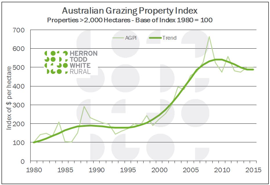
Figure 1. Australian Grazing Property Index (Source: RP Data and Herron Todd White (2015)).
Seasonal conditions
For many in agriculture the seasonal conditions are the biggest single driver of performance and ultimately the relative value of land. When the rain fell, how much soil moisture was contained within the soil profile, was the growing period affected by short cold winter or long hot summer all affect the performance of the business. The variability of seasons suggests that investment decisions should be made using the average performance of the operation over say five years, to account for this variability.
The question then arises that, if due to seasonal circumstances the average return over an agreed period of time is a loss, what does this suggest in regard to the value of the underlying asset? The asset still consists of productive land (when it rains) which includes housing and infrastructure and other features.
Table 3 reflects eight years of performance results in the West Australia Planfarm Bankwest benchmark series. The results highlight that the top 25% of operators on average, strongly outperform the remaining 75% with no negative returns in the eight years. In comparison, the average operators had two negative years in eight and one just above breakeven, whereas the bottom 25% had six negative performance years in eight. This data is from 566 farm businesses throughout broadacre farming regions in WA (Figure 2).
| 2007 | 2008 | 2009 | 2010 | 2011 | 2012 | 2013 | 2014 | Average | |
|---|---|---|---|---|---|---|---|---|---|
| Top 25% | 16.05% | 20.12% | 4.26% | 4.24% | 11.80% | 5.26% | 15.34% | 9.78% | 10.11% |
| Average | 6.08% | 7.05% | -1.38% | -1.00% | 7.16% | 1.07% | 8.17% | 5.00% | 3.73% |
| Bottom 25% | -4.70% | -1.90% | -6.70% | -6.35% | 2.24% | -4.16% | 0.46% | -0.71% | -2.45% |
(Source: Planfarm Bankwest Benchmarks 2014/2015 (2016)).

Figure 2. Return on capital for WA broadacre farms. (Source: Planfarm Bankwest Benchmarks 2014/15 (2016)).
The top 25% in the eight years delivered a very impressive 10.11% return. The top 25% are not necessarily the same businesses in the same region each year. The return from the average producers falls very quickly to 3.73%. The performance of the average group of 3.73% is lower than the average cost of debt during this same period.
During this same period the median land price per hectare as represented in Figure 3 (All WA) moved from $1108 per ha up to a peak at $1205 per ha in 2011 and subsequently fell to $1102 per ha. So the overall land appreciation over this period has largely been nil. For south western WA the story is a bit better with the median price of land moving from $1055 per ha to $1351 per ha (+28% growth in value in eight years). There were approximately 1400 property sales in that time period (Figure 4).
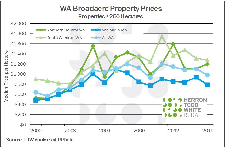
Figure 3. WA broadacre property prices, properties > 250 hectares. (Source: RP Data and Herron Todd White (2015)).
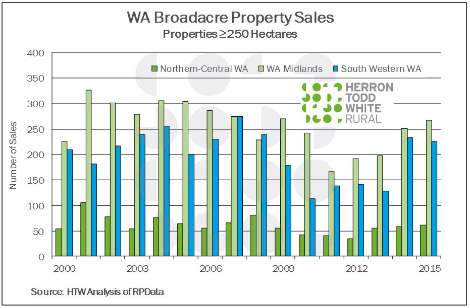
Figure 4. WA broadacre property sales, properties > 250 hectares. (Source: RP Data and Herron Todd White (2015)).
It may be possible to gain district data of average yields via the processing facilities, or benchmarking data sets as reflected in the WA figures. This analysis is based on 566 farm businesses throughout the broadacre farming regions in WA. The use of benchmark data is good to understand relative performance but if the actual financial performance of the particular property being valued is only seen by the owner, their accountant and the friendly banker, the valuer has no insight into this aspect. What does clearly get highlighted is that the top 25% of operators in the survey generate very good returns overall, and therefore, the question becomes why? Scale, management decisions, education and experience, enterprise combination, location, seasonal conditions all add to the mix in this regard.
The management of any business has a critical impact on the overall business performance and agriculture is no different. For a cropping business, timeliness is critical to yield, and therefore, returns. A focus on input costs versus return also needs to be soundly based. The best yielding crop may not actually deliver a better overall year end outcome. It is a bit like the grazing business owner who seeks to top the sale with an animal but loses sight of the cost to carry that animal to that point and at some time the net return beyond a point of growth could be at diminishing margins. The decisions about for example, pasture management (whether to sell off and buy back in) and spending on fodder to hold a line of genetics all factor into the final profit and loss result year in and year out.
If financial return was the sole focus, the decisions made by many operators would vary to those previously made.
The other side of an income approach question is what is the capitalisation rate that should be applied to the return to reflect the value.
The capitalisation rate, often just called the cap rate, is the ratio of net operating income (NOI) to property asset value (Figure 5). So, for example, if a property sold for $1,500,000 and generated a NOI of $100,000, then the cap rate would be $100,000/$1,500,000, or 6.66%.

Figure 5. Equation to calculate the capitalisation rate.
Intuition behind the cap rate
What is the cap rate actually telling you? One way to think about the cap rate intuitively is that it represents the percentage return an investor would receive on an all cash purchase (Table 4).
Cap rate | 12.00% | 11.00% | 10.00% | 9.00% | 8.00% | 7.00% | 6.00% | 5.00% | 4.00% |
|---|---|---|---|---|---|---|---|---|---|
Multiple | 8.33 | 9.09 | 10.00 | 11.11 | 12.50 | 14.29 | 16.67 | 20.00 | 25.00 |
So with an average annual return of 3.73% in the WA example the multiple is 26.8 times earnings.
Buyer motivation and locational advantage
Another key aspect of the agricultural land market is the motivation of the buyer in the transaction. Unlike a commercial property investment which is much more focused on the yield, tenant risk and outgoings for example, a buyer of agricultural assets may also be motivated by non-commercial aspects to some degree.
A son or daughter returning home to the farm can be a catalyst for acquisition. The investment, if made on a purely standalone basis, may not be viable. However when coupled with surplus income from the existing operation, the provision of a housing solution and the potential to gain greater efficiency from current machinery, the transaction may become viable and bankable.
To highlight this point that there other aspects that motivate buyers, the Queensland Rural Adjustment Authority (QRAA) completed a bi-annual debt survey and the 2009 summary of debt and gross value of production (GVP) provides a good insight into the potential return profile of rural Queensland agricultural businesses (Table 5). In the 2007 review period debt to agriculture increased 36.30% and GVP fell 2.07%.
Year | Total debt $’000 | Debt as % of GVP (%) | GVP $’000 | Yearly % increase in debt (%) | Yearly % increase in GVP (%) |
|---|---|---|---|---|---|
2009 | 15,061,972 | 168.5 | 8,939,000 | 27.42 | 7.76 |
2007 | 11,820,465 | 142.5 | 8,295,000 | 36.30 | -2.07 |
2005 | 8,672,315 | 102.4 | 8,470,000 | 12.53 | 16.94 |
2003 | 7,706,691 | 106.4 | 7,243,000 | 15.65 | -0.04 |
2001 | 6,663,555 | 92.0 | 7,245,627 | 6.32 | 7.02 |
2000 | 6,267,652 | 92.6 | 6,770,652 | 6.74 | 6.13 |
1999 | 5,871,748 | 92.0 | 6,379,713 | 11.10 | 8.96 |
1998 | 8,285,061 | 90.3 | 5,854,874 | 9.52 | 3.13 |
1997 | 4,825,535 | 85.0 | 5,677,093 | 2.16 | 6.72 |
1996 | 4,723,330 | 88.8 | 5,319,670 | 16.09 | -2.68 |
1995 | 4,068,668 | 74.7 | 5,466,416 | 5.01 | 4.98 |
1994 | 3,874,471 | 74.4 | 5,206,927 |
n.b. The debt for the 2000 year has been calculated, based on a prorate movement between the 1999 and 2001 years. (Source: QRAA – Survey Results (2009)).
In the same two year period from 2005 to 2007 the median dollar value per hectare as measured by the Herron Todd White Queensland broadacre property prices (greater than 250 hectares) moved from $923/ha to $1225/ha (an increase of 32.7%) (Figure 6).

Figure 6. Queensland broadacre property prices, properties >250 hectares. (Source: RP Data and Herron Todd White (2015)).
In 2011, the survey report is in a different format showing the proportion of debt to GVP and the gap continues to widen on a gross basis (Figure 7). During the two years from 2009–11 the median price per hectare of land did shift down from $1316/ha to $1188/ha, a 10% reduction. This reduction in value is still on an increasing debt level to agriculture and as reflected in Table 6 is in part a function of the reduced GVP for beef and grain and grain/grazing.

Figure 7. Debt levels versus gross value of production estimates. (Source: Queensland Rural Adjustment Authority (2011)).
Percentage movement in debt | Percentage movement in GVP | |
|---|---|---|
Beef | 17.2% | -4.9% |
Cotton | 36.9% | 156.5% |
Grain and grain/grazing | 25.3% | -19.8% |
(Source: Queensland Rural Adjustment Authority (2011)).
The impact of commodity price fluctuations
The final variable for this topic is then the commodity price itself. Australia is an export orientated producer of agricultural products. Approximately 65% of our agricultural production is exported, and therefore, we remain susceptible to global supply and demand changes along with currency movement risk which impacts our price competitiveness. This volatility is reflected in Figure 8, which uses the beef sector to highlight the variability over 30 years.
For those then looking to model the income side of a return equation, what is the best assessment to base assumptions for performance upon? Agriculture has largely been a price-taker and while there is some shift in this with some forward selling and hedging options in some commodity classes, the ability to better manage the income from operations remains a key factor in final outcomes.
Commodity prices are largely related to global production and it has proven extremely difficult to forecast this, given the impact of seasonal conditions and government policy in our key export markets (Figure 8). Both of these factors are difficult to predict, and yet in many respects have the greatest influence on prices. The recent signing of free trade agreements with some of our main export countries has the potential to reduce the volatility.

Figure 8. Northern cattle market from 1986 to March 2016. (Source: Bush AgriBusiness analysis (2016) using data from MLA’s NLRS and ABS).
Conclusion
Overall it is hard to show a clear correlation between investment return and land values on a year in, year out basis. As a pure investment the return if operated in isolation may not be viable and this is specifically evident for smaller-scale holdings which do not attract institutional capital. The big end of town holdings require a scale of operation that allows for independent management and return as there is no cross-subsidisation of the transaction from other assets. Corporate capital with investment discipline requires a regular return and it is one of the reasons that investment into the Australian agriculture has been a challenge.
The opportunity for this capital to buy an asset and be the lessor to good farm managers who can benefit from the efficient use of working capital does represent a potential business outcome that brings together good capital and good operators for a mutual benefit. The development of this model is not new globally with the United States and Europe having a high percentage of land ownership outside of the farming business (either family or corporate managed). The Australian market place is starting to see this growth in a lessor/lessee model, however determining the lease rates that support a viable operator and meet investment outlooks is still a challenge.
The falling global bond rates and cash rates in Australia, now down to 1.75%, will assist investors looking for return to think about rural land as a longer-term place to invest. A long-term earnings of 4% coupled with approximately 5% long-term capital growth is still a good outcome for most investment. The investment term however becomes critical given the long cycle of agriculture in land values (approximately 18 years for a full cycle when looking at the Australian Grazing Property Index (AGPI) graph).
So for the valuer, it is back to the original question. The fundamental basis for assessment remains a comparison to other like assets within the locality, understanding these sales and the analysis of these sales on a productive unit basis for livestock, dollars per AE/DSE/Bird/CSU – for feedlots, etc. At least that way the relativity between two properties can be determined and if the sales analysis is consistent, the outcome should be a good representation of the market.
The valuer’s role is to interpret the market and sales transactions, the buyers and sellers of the assets set the market and the pricing. The return assessment in all transactions needs to be satisfactory for both parties however whether this meets an acceptable investment return remains a topic for ongoing debate. A valuer is obligated to adhere to the accepted valuation principles and apply the most appropriate method of assessment to the asset while having regard for the client’s instruction and also the concept of basing the value on the property’s highest and best use. The valuer needs to understand why a particular buyer paid a particular price for a property or why the vendor sold the property for a particular price, hence why the job of interpreting value through drawing conclusions through correct comparison techniques (which only comes with experience) is very subjective. Valuation is often referred to as an ‘inexact’ science.
Figures 9 and 10 (not the same property), highlight the variability of the sector and the need for caution when looking at investment return as a measure of land value.

Figure 9. North West Queensland, February 2016.

Figure 10. North West Queensland, April 2016.
Acknowledgements
For their expert opinion and overview: Douglas Knight – Certified Practising Valuer, Toowoomba; Graeme Whyte – Certified Practising Valuer, Mildura; and Michael Gannon – Certified Practising Valuer, Brisbane.
References
ABARES (2011), Australian Farm Survey Results 2008–09 to 2010–2011, ABARES, Canberra.
Bush AgriBusiness (2016), Real Queensland Cattle Prices, Current to September 2014, Withcott, Queensland.
Planfarm (2016), Planfarm Bankwest Benchmarks 2014/2015, Floreat, Western Australia.
RP Data and Herron Todd White (2015) national rural market update.
Queensland Rural Adjustment Authority (2009 and 2011), 2009 and 2011 Rural Debt Surveys, Queensland Government, Brisbane, Queensland.
Contact details
Tim Lane
tim.lane@htw.com.au
Was this page helpful?
YOUR FEEDBACK