Take home messages

• Financial leverage, or gearing, refers to the use of borrowed funds for additional asset acquisition. The aim is to increase the rate of return from the investment by amplifying the return over a greater value of assets under management. High levels of leverage or gearing mean that a business is carrying high debt to equity ratios.
• Financial leverage can be a useful way to increase wealth in agriculture but there are associated risks. Understanding leverage, how it works, and the risks involved can help to make informed judgements about its application within the business.
• In agriculture, leverage is typically used to expand farm operations by utilising equity in an existing asset portfolio and purchasing additional land. This paper looks at what financial leverage is and how it helps to create wealth.

An example demonstrating how leverage works

An example of how leverage works is provided in Table 1. The first data column of Table 1 (‘Unleveraged’) details the workings of an unleveraged investment with $100,000 of equity. Data column 2 (‘Leveraged’) shows the workings of a leveraged investment with the same amount of equity but additional borrowings. The assumptions driving the outcomes shown in Table 1 include an interest rate of five percent on borrowed funds and a total investment return of ten percent.

The results demonstrate how a leveraged investment generates greater returns on equity than an unleveraged investment where the cost of capital is lower than the return on investment.

Table 1. Comparison of an unleveraged investment with a leveraged investment.

An unleveraged investment

Data column 1 of Table 1 (‘Unleveraged’) demonstrates the return on investment without the use of leverage. Equity of $100,000 has been invested, but no debt has been utilised. This means that the equity invested equates to the total value of the investment. The return from this investment is 10 percent which generates $10,000 on the $100,000 invested. There is no debt so there is no cost of debt funding thus the net return on equity is 10%.

A leveraged investment

The leveraged investment is shown in data column 2 of Table 1 (‘Leveraged’). In this example $100,000 of equity is invested but in addition to this investment $900,000 of debt has been borrowed bringing the total investment amount to $1 million.

Leverage in this example is a debt to equity ratio of 9 to 1. This means that for every dollar worth of equity in the investment nine dollars-worth of debt has been incurred. In other words, of the total million-dollar investment $100,000 was raised from equity. The remaining $900,000 was borrowed. This may be called a 90 percent leveraged investment.

The total profit generated by the leveraged investment has been calculated by multiplying the assumed ten percent return on the million-dollar investment equating to $100,000. This is a ten-fold increase in profit before interest relative to the unleveraged investment. Unlike the unleveraged example however, interest costs are incurred on the $900,000 of borrowings relating to an additional cost against this investment.

The annual cost of interest on the debt is calculated by multiplying the interest rate of 5% by the debt of $900,000. The annual cost of interest equates to $45,000.

Profit after interest is calculated by deducting the interest cost from the profit. Thus, the outlay of $100,000 in equity results in a net return of $55,000 which equates to a return on equity of 55%.

Key point – leverage works where the return from debt exceeds its cost

This comparison of leveraged versus unleveraged investment shows that the rate of wealth creation is far higher with a leveraged investment relative to an unleveraged investment provided the investment return exceeds the interest rate.

The cost of funds or the interest rate on borrowed capital is an important factor driving the outcome of the analysis. Leverage creates wealth for investors only where the investment return exceeds the cost of borrowed funds (the interest rate). If the interest rate exceeds the rate of return generated by the investment, then the investment erodes wealth rather than creating it.

Sensitivity

Figure 1 shows that leverage is highly sensitive to the rate of return on investment. The net return of the leveraged investment after interest costs are accounted for fluctuate from -$25,000 at two percent investment return to $35,000 at eight percent investment return.

This demonstrates that leverage erodes wealth when the interest cost exceeds the total investment return. At an investment return of two percent and an interest cost of five percent each dollar borrowed is losing three percent. This means that a $27,000 loss is incurred on the $900,000 of debt. The equity still generates two percent return but given the equity component is only $100,000 of the total investment the equity component of the investment returns only $2,000. This delivers a net loss of $25,000 on the total million-dollar investment where returns decline to two percent.

Where the investment return is higher than the cost of interest more wealth is created with the combination of debt and equity funding compared with equity funding alone. The return is dependent on the margin between the investment return and the cost of debt funding and the magnitude of the debt funding.

For example, the net return on debt where the investment return is 8% is only 3% (the difference between the return and the interest cost) but it is generated on $900,000. This provides the majority ($27,000) of the $35,000 return. The remaining $8,000 comes from the equity component.

Where the return generated from the investment exceeds the cost of interest (5%) a positive return is generated. Where the cost of debt funding is equivalent to the investment return there is no net gain on the debt and a net return of 5% on the equity. This is why the net return is equivalent to the non-leveraged investment at this point. The assumption is that the debt to equity ratio of the investment is 9 to 1.

The unleveraged investment does not deliver the same degree of volatility in profits as does the 90 percent leveraged investment because the gross value of the unleveraged investment equates to only one tenth of the value of the leveraged investment.

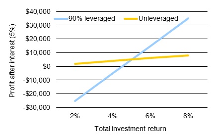
Figure 1. Leveraged wealth creation is dependent on the margin between the return on investment and debt funding.

Figure 2 demonstrates the sensitivity of profits to investment returns at high levels of leverage. On a million-dollar investment at interest costs of five percent, 90 percent leverage and two percent investment returns, the extent of the losses on the debt dwarfs the value of the profits on the equity. The same investment at interest costs of five percent, 90 percent leverage and eight percent investment returns, generates large profits on the debt but proportionally larger profits on the equity due to no costs being incurred on the equity component.

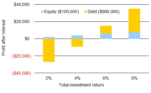
Figure 2. The higher the leverage the higher the risk exposure to low returns.

Case study 1 - $5 million in asset value at 70% starting equity

A case study has been conducted to investigate the theory of leverage in practice. A business with $5 million in total asset value at 70 percent equity was modelled over a ten-year period. Average interest rates of 6% were imposed and sensitivity to returns analysed. The business is assumed to reinvest capital at a rate of $50,000 per year to replace depreciated plant and equipment. Volatility of returns is an important consideration, but it has not been addressed in this comparison.

The three following investment scenarios were assessed:

1. Debt reduction – after tax cash profits go to reducing debt.
2. Conservative growth – after tax cash profits are invested in as much additional farming land as can be acquired at the going land price. If cash losses occur, then no purchases are made and liabilities are assumed to increase. This is an unrealistic situation run only to establish the relative return.
3. Aggressive growth – after tax cash profits plus any increases in equity due to capital gain are invested in as much additional farming land as can be acquired at the going land price. Land is still purchased if cash losses occur but only by the magnitude of the value of the gain in equity less the value of the cash loss.

The outcome

Where operating returns equate to two percent and capital growth equates to four percent there is little difference between growth strategies (Table 2). No scenario generates free cash thus no cash investment is made into additional land or into repaying debt. The aggressive strategy continues to purchase land using accumulated equity however in reality the average interest cover ratio of less than one is unlikely to facilitate the availability of debt for leverage.

The aggressive strategy delivers no more wealth and less cash than the alternative strategies because the cost of debt on hectare of additional land leveraged is the same as the value of the return generated from that land. Cash reserves are lower because the operating return of two percent is inadequate to cover the cost of interest (6 percent). The wealth created is similar because the return on debt is similar to the return generated from

Table 2. Differences between growth strategies where operating returns equate to two percent and capital growth equates to four percent.

Where operating returns increase to four percent and capital growth remains at four percent then the most aggressive of strategies creates marginally more wealth than the remaining strategies (Table 3). More debt in the aggressive strategy leads to less cash however this is more than offset by the additional capital growth.

The debt reduction strategy leads to lower returns than the alternatives as the interest cost is only six percent. The alternatives, where free cash or free cash plus equity are invested generate four percent operating plus four percent capital gain.

As operating and capital returns exceed these levels then the magnitude of the difference in strategies is only further exacerbated in favour of the aggressive strategy.

Table 3. Differences between growth strategies where operating returns equate to four percent and capital growth equates to four percent.

Case study 2- $8 million in asset value at 44% starting equity

An additional case study has been conducted to investigate the theory of leverage in practice. A business with $8 million in total asset value at 44 percent starting equity was modelled over a ten-year period. Average interest rates of 6% were imposed and sensitivity to returns analysed. The business is assumed to reinvest capital at a rate of $65,000 per year to replace depreciated plant and equipment. Volatility of returns is an important consideration, but it has not been addressed in this comparison.

The same three following investment scenarios including debt reduction, conservative growth and aggressive growth were assessed.

At two percent operating return and four percent capital growth the cash losses exceed $2 million regardless of which strategy is followed. Such a level of cash loss is unlikely to be tolerated without an expectation of liquidation of some assets to reduce liabilities.

Where operating returns increase to four percent and capital growth remains at four percent then the most aggressive of strategies still creates more wealth than the remaining strategies (Table 4). More debt in the aggressive strategy again leads to less cash however this is still more than is offset by the additional capital growth.

The debt reduction strategy again leads to lower returns than the alternatives as the interest cost is only six percent. The alternatives, where free cash or free cash plus equity are invested generate four percent operating plus four percent capital gain.

The debt reduction strategy and the conservative strategy both lead to growth in equity over time primarily due to the accumulation of capital gains. The aggressive strategy does not allow capital gains to accumulate as equity rather it uses leverage against that equity to expand and purchase more land.

Table 4. Differences between growth strategies where operating returns equate to four percent and capital growth equates to four percent.

Other issues not identified in these case studies

The outcomes of these case studies reinforce the theory of the use of leverage. Debt can assist in creating wealth in agriculture but only where the returns from that debt exceed its cost.

The outcomes of these analyses are not an endorsement for any strategy but rather they use scenarios to demonstrate the relative rate of wealth creation using debt. Personal risk profiles and comfort levels will play a major role in the level of financial leverage assumed in a business. Some business operators are comfortable with the aggressive strategy while others are happy with the debt reduction strategy. Understanding the differences between them is the key.

Regardless of comfort levels, exit strategies should be developed at the point of acquisition. While any forced liquidation will drive a level of discomfort, executing the exit strategy is akin to executing an insurance policy. It will come at a cost but that cost offsets a far more significant loss.

Volatility is real but hasn’t been presented in these case studies. Volatility in returns can readily be projected by assessing the range in operating returns over the last decade. This is where having a solid set of management accounts or a record of benchmarking really adds value. In areas where returns are volatile then the rules can change. They change because greater cash reserves will be necessary to get through consecutive poor seasons.

What this means to you

Agriculture is a business particularly well suited to the use of financial leverage. High equity levels in an existing business can be used to leverage and create wealth through expansion. Leverage allows for a greater rate of wealth creation than using equity alone provided the net investment return exceeds the cost of debt funding. Understanding the volatility of returns and the risks involved in highly leveraged situations is still important as any strategy that starves a business of cash is more likely to destroy rather than create wealth.

Contact details

John Francis
Holmes Sackett
john@holmessackett.com.au