Break crops can form part of a profitable cropping system in the low rainfall zone of Western Australia

Key messages

• Break crops, such as canola and pulses, can be part of a profitable crop rotation in the low rainfall zone (LRZ).
• When analysed at the level of a single paddock at a single year, wheat is the most profitable and least risky crop to grow in the LRZ.
• However, when analysed at the whole farm level over multiple years (that include break effects and diversification effects) rotations including break crops can be as profitable and less risky than continuous wheat.
• Farmers need to identify which break crops fit their soils, climate and farming systems. They then need to optimise their agronomy to maximise profitability.

Aims

Our aims were firstly to test whether high-value break crops can be grown profitably in the LRZ (low rainfall zone) and secondly to conduct an economic analysis to determine how break crops contribute to the overall profitability and risk of cropping in the LRZ.

Introduction

Determining which crop to grow and in what sequence is a complex decision. At the most basic level, farmers weigh up the expected yield of a crop, the expected input costs and the expected price to calculate an expected gross margin. However, there are many interactions and variables that complicate the choice of crop:

• There is a clear yield benefit from crop rotation. Wheat growing after a non-cereal crop will usually yield more due to a break in weed and disease cycles and any additional nitrogen supplied (especially if the break crop is a legume). For example, using experimental data Seymour et al (2012) showed that wheat yields in WA grown after lupins had a 0.6t/ha yield benefit compared to wheat grown after wheat. Therefore, farmers may accept a small loss in profitability in one year if they can regain it in a following crop.
• There is year-to-year variation in both yield and price that cannot be predicted at sowing. Therefore, growing more than one crop is likely to be useful to diversify income streams. Diversified cropping rotations have been shown to be more resilient than those that are heavily reliant on a single crop (Lawes and Kingwell 2012). Furthermore, diversified income on farm has been shown to reduce risk (e.g. Bellet al 2021).
• Grain prices are also variable. For example, WA wheat prices have ranged between $195 and $389/t over the past 20 years and canola prices have ranged between $300 and $580/t (Australian-Bureau-of-Statistics 2017). Again, growing more than one crop is likely to be useful to diversify income streams and mitigate price risk.

The LRZ of WA has low uptake of break crops likely due to weather variability at the cropping margins and the perceived risk of many alternative crops, especially legumes (Fletcher 2019). Canola is the largest non-cereal break crop in the LRZ occupying about 11% of the cropped area (Planfarm:BankWest 2016), due to the high prices this crop receives relative to other non-cereal options, and the many herbicide options available, which aid in weed control. Lupin is the largest legume crop occupying 6% of the cropped area due to its adaption to the sandy acidic soils prevalent in much of WA. However, low prices are likely limiting the area of lupins grown. Farmers require information about the profitability of various break crop options. More importantly, profitability needs to be assessed in multiple paddocks and across multiple years given the seasonal variations in weather and grain prices.

We report the results of three field experiments that compared the yield and gross margins of a range of legume break crops. We then calculated yields and profitability for wheat and a range of alternative crops in the LRZ using industry data. We used these data to compare the mean gross margins and risk of a range of potential cropping rotations. We accounted for both the break crop benefit to subsequent wheat crops and the income diversity from having multiple crops. We also discuss how the yields of break crops can potentially be improved with a range of agronomic management practices to further increase their value in crop rotations.

Methods

Field experiments

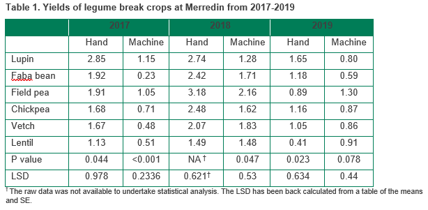
Field experiments were carried out at Merredin over three consecutive years (2017-2019). In each experiment six potential legume break crops were sown at their recommended sowing rate. The legume crops were ‘PBA Jurien’ lupin; ‘PBA Samira’ faba bean; ‘PBA Gunyah’ field pea; ‘PBA Striker’ chickpea, ‘PBA Volga’ vetch; and ‘PBA Bolt’ lentil. In 2017, the trial was sown on 6 May on a loam soil following a canola crop in 2016. In 2018 the trial was sown on 1 June on a clay soil following a fallow in 2017. In 2019 the trial was sown on 22 May on a loam soil following a wheat crop in 2018. Growing season rainfall (Apr to Oct) was 195mm, 218mm and 202mm in the three years respectively. Grain yields were obtained by hand harvests and small plot machine harvester.

Gross margins of experimental results

We calculated the economic return of each crop. Partial gross margins were calculated using the yields (hand harvest), variable costs of growing each crop (which did not vary between seasons) and a constant grain price. We did not consider fixed costs at the farm level, (e.g. machinery or land costs). The costs for growing each crop were calculated as $188/ha for lupin, $254/ha for faba bean, $209/ha for field pea, $275/ha for chickpea, $170/ha for vetch and $202/ha for lentil. Grain prices were $330/t for lupin, $450/t for faba bean, $429/t for field pea, $776/t for chickpea, $529/t for vetch and $568/t for lentil. In each year, gross margin data are presented relative to the crop with highest gross margin. We acknowledge the prices vary substantially between years but that these prices represent five-year averages between 2016 and 2020.

Economic analysis of rotations

We analysed the economics and risk at both the farm level and across multiple years. This is similar to the approach used by Lawes and Renton (2010) using the LUSO model. However, our approach differed in two key ways:

1. We did not attempt to keep track of weed and pest populations or soil nitrogen. Instead these were accumulated into a single break crop effect (Seymouret al 2012); and
2. We did not use long-term mean yields and prices, instead we calculated variable yields and prices that varied from year-to-year.

We calculated gross margins for 13 rotations detailed in Table 3.

We used the following costs for growing each crop: continuous wheat (with ryegrass weed issues) - $202/ha, wheat after canola - $160/ha (accounts for reduced herbicide costs), wheat after legume crop - $137/ha (accounts for reduced herbicide and N costs), barley - $168/ha, oats - $172/ha, canola - $175/ha (this rose to $192/ha in 30% of years to account for outbreaks of diamond back moth that required an extra pesticide spray), lupin - $188/ha, field pea - $209/ha and chickpea - $275/ha.

Wheat yield data were taken from the Planfarm Bankwest data set between 2000 and 2018. This provided wheat yields for 1544 farm-by-year combinations in the LRZ. We then calculated a population of yields of the other crops from the regressions of Fletcher (2019) and the associated variation with each regressions. This was necessary because not every crop was grown on each farm in the original data set. We also calculated wheat yields that accounted for the break crop effect. i.e. wheat after a break crop yielded more than continuous wheat using the relationships of Seymouret al (2012) and the associated variation with each regressions, i.e. the break crop effect was not consistent and varied between years as it would on-farm. The implicit assumption was that all soils could grow all crops.

We also calculated a population of grain prices for each crop using ABS data (2000-2019) and the relative relationships between each commodity were maintained, e.g. wheat and barley prices were closely linked but the prices of wheat and chickpea were only poorly linked reflecting the higher volatility of chickpea prices.

From this population of yields we calculated partial gross margins for 1) comparing single paddocks of each crop, 2) rotations in a single paddock accounting for break crop effect, (i.e. wheat grown after a break crop had increased yield, 3) multiple paddocks across single years (only accounting for the diversification effect and not accounting for the break crop effect) and 4) multiple paddocks over a rotation (accounting for both the diversification and break crop effects).

Results

Legume break crop trials

In each year of the experiments there were significant differences in yield between crops. Lupin was consistently high yielding and lentil was consistently low yielding (Table 1). Field pea gave the highest yields in 2018 but had only intermediate yields in the 2017 and 2019. In general, for all crops, the hand harvested yields were greater than the machine harvested yields. This indicates that harvestability of these crops may be an issue limiting adoption.

When the yields from these trials were converted to gross margins the outcomes were quite different. The relative returns of each crop are shown in Figure 1. The data for each year were scaled to the crop that gave the highest returns in each year. Overall, chickpea consistently generated the highest returns. In 2017, chickpea delivered the highest return of $733/ha, in 2018 field pea gave the highest return of $1242/ha, and in 2019 chickpea generated the highest return of $421/ha. Lentil had consistently poor returns compared to the other crops. Field pea was more variable giving high returns in 2017 and 2018 but comparatively poor returns in 2019. Despite having consistently high yields (Table 1), lupin delivered only low to medium returns. These results highlight that chickpea warrants further research and development in the LRZ. In particular the agronomy and fit within a cropping system should be explored. For example, Rich and Lawes (2020) demonstrated that chickpeas can emerge and yield well from sowing as deep as 200mm and that sowing these crops early can markedly increase yield.

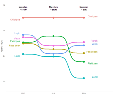
Figure 1. Calculated partial gross margins (using hand harvest yield data) for six grain legumes in Merredin over three years. In each year, the data are scaled to the crop that gave the highest gross margin in that year.

Rotation economics

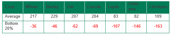
Table 2 shows the mean gross margins and the mean gross margin in the bottom 20% of years calculated for each crop in the analysis. This shows that when only the costs, price and yield of each crop are considered, wheat and barley are the most profitable and the lowest risk crops to grow in the LRZ. This probably explains the dominance of these two crops in the LRZ. It also explains the low uptake of legumes crops due to their higher risk. However, this analysis does not account for the income diversification and break crop benefits that may accrue at the rotation and farm level.

Table 2. Calculated partial gross margins ($/ha) of individual crops in the LRZ. The mean gross margin for each crop is shown as a measure of overall profitability, the mean gross margin in the bottom 20% of years is shown as a measure of risk.

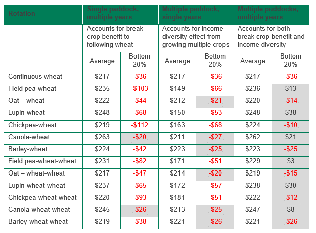
When the break crop effect to the following wheat crops was included, (i.e. a single paddock followed over multiple years) most rotations gave slightly higher average gross margins than wheat (Table 3). However, with the exception of the canola-based rotations, continuous wheat was still the lowest risk. In particular the legume-based rotations were still far more risky than continuous wheat. These results likely account for the prevalence of canola as the major break crop in the LRZ of WA. These results also demonstrate that the break crop effect on its own is not a compelling reason to include legumes in LRZ cropping rotations.

When only the diversification effect was included, (i.e. multiple paddocks were evaluated for a single year) the rotations that included barley, canola or oats had similar average returns to continuous wheat but reduced risk (Table 3). When both the break crop effect and diversification effect were included, (i.e. multiple paddocks were evaluated over multiple years) the outcome was quite different. The average return of all sequences was slightly greater than continuous wheat. More importantly, the risk was also reduced especially in legume- and canola-based rotations. Under this scenario continuous wheat was the most economically risky rotation.

These results came about for several reasons. Wheat growing after break crops had improved yield. This has the effect of improving the overall average profitability of wheat but also increasing yield in the poor years. Wheat crops grown after legumes and canola had reduced costs, which helped to reduce economic risk. Farms with multiple crop types had diversified income streams, which helped to mitigate the effects of poor yields (due to a number of factors) or poor prices of a single crop.

Table 3. Calculated partial gross margins of rotations in the LRZ. The mean gross margin for each rotation is shown as a measure of overall profitability, the mean gross margin in the bottom 20% of years is shown as a measure of risk. In each scenario, rotations that are less risky than continuous wheat are highlighted.

This analysis has several limitations that may affect the gross margins calculated but is unlikely to impact the overall outcome. The first is that the analysis assumes that all crops can be grown on all soils. This is clearly not the case and each farmer will need to adjust their choice of break crop depending on soil. The second limitation is that we assumed the costs of growing each crop were fixed. In reality, farmers in the LRZ are skilled practitioners and adjust costs (particularly fertiliser) to match likely crop yield. The third limitation is that our rotations are relatively simple in that they rotate only a single break crop with wheat, and do not account for double-break rotations that are becoming more common in the LRZ. The fourth limitation is that the analysis did not allow for break crop effects that extend beyond a single season (e.g. Kirkegaard and Ryan 2014). This would make the analysis more favourable to break crops. The fifth limitation is that the rotations are fixed. Many farmers in the LRZ are skilled at adjusting rotations to climatic conditions. For example, farmers may sow more canola when there is an early break. In particular our analysis does not include fallow. However, the economics of fallow need to be evaluated as a strategic management (Oliveret al 2010).

Conclusion

Our results have shown that break crops can be grown profitability in the LRZ of WA.

Furthermore, our analysis has shown that break crops can form part of a profitable rotation in the LRZ.

Our aim here was not to recommend one break crop over another but rather to demonstrate that when the economics are viewed in terms of both the break crop benefit to subsequent wheat crops and the value of income diversification, the outcome can be quite different from a simple gross margin of each crop. Farmers need to consider both the rotational benefits and the diversification benefits when considering new break crops.

Acknowledgments

This research was jointly funded by GRDC and CSIRO as part of the low rainfall zone project (CSA00056). We thank the CSIRO technicians for assistance with completing the field experiments. The research undertaken as part of this project is made possible by the significant contributions of growers through both trial cooperation and the support of the GRDC, the authors would like to thank them for their continued support.

References

Australian-Bureau-of-Statistics (2017).7503.0 - Value of Agricultural Commodities Produced, Australia, 2016-17.

Bell, L. W., Moore, A. D. & Thomas, D. T. (2021). Diversified crop-livestock farms are risk-efficient in the face of price and production variability. Agricultural Systems 189: 103050.

Fletcher, A. (2019). Benchmarking break-crops with wheat reveals higher risk may limit on farm adoption. European Journal of Agronomy 109: 125921.

Kirkegaard, J. A. & Ryan, M. H. (2014). Magnitude and mechanisms of persistent crop sequence effects on wheat. Field Crops Research 164: 154-165.

Lawes, R. & Renton, M. (2010). The Land Use Sequence Optimiser (LUSO): A theoretical framework for analysing crop sequences in response to nitrogen, disease and weed populations. Crop and Pasture Science 61(10): 835-843.

Lawes, R. A. & Kingwell, R. S. (2012). A longitudinal examination of business performance indicators for drought-affected farms. Agricultural Systems 106(1): 94-101.

Oliver, Y. M., Robertson, M. J. & Weeks, C. (2010). A new look at an old practice: Benefits from soil water accumulation in long fallows under Mediterranean conditions. Agricultural Water Management 98(2): 291-300.

Planfarm:BankWest (2016).Planfarm Bankwest Benchmarks 2011-2016.

Rich, S. & Lawes, R. A. (2020).Sowing flexibility of chickpea and lentil in the Western Australian farming system. In GRDC Research UpdatesPerth: GIWA.

Seymour, M., Kirkegaard, J. A., Peoples, M. B., White, P. F. & French, R. J. (2012). Break-crop benefits to wheat in Western Australia – insights from over three decades of research. Crop and Pasture Science 63(1): 1-16.

Contact details

Andrew Fletcher
CSIRO
Private Bag 5 Wembley, WA 6913
Phone: 08 9333 6467, 0477 347 449
Email: andrew.l.fletcher@csiro.au