AgScore: A form guide for selecting the best climate model to use - how accurate are different climate models in different regions and situations?

Take home message

• The regional inter-model comparison of 12 seasonal forecast systems showed that no single forecast system stood out as superior in predicting rainfall for all regions and seasons. However, our analysis did identify groups of models having skill, particularly in winter and spring
• The Bureau’s model (ACCESS-S1) was consistently one of the top performers across most of eastern and northern Australia based on our regional analysis
• A more in-depth evaluation of wheat yield forecasts generated from the top performing forecast systems indicated sufficient skill from mid-way through the season (July). This implies that at best, seasonal climate forecasts can provide guidance on yield estimates during the middle to latter stages of the winter growing season.

Introduction

The AgScore project represents a new approach to a pertinent question in agri-climatology: How good is my seasonal climate forecast? Seasonal climate forecasts (SCFs) can provide important information and can reduce agricultural decision-making risk, provided they are timely, relevant and accurate (Meinke et al., 2006). Seen as a critical innovation for farming in the last three decades, the uptake of SCFs is increasing but still faces major challenges particularly around their quality and usefulness (Hayman et al., 2007; Taylor, 2021).

The agricultural sector is one of the largest users of SCFs, particularly for farming systems that are dependent on seasonal patterns of rainfall e.g., grains and livestock industries (Centre for International Economics, 2014; Robertson et al., 2016). A skilful SCF can mean many different things depending on the user and how the forecast information affects their decision-making process. Agriculturally relevant forecasts can include climate-based predictions for specific time windows or relevant thresholds (e.g., probability of receive in excess of 20 mm in the next month) and more sophisticated predictions of yield or farm productivity (Cowan et al., 2020; Hansen et al., 2004).

A central premise of the AgScore project is that the evaluation of seasonal climate models, and the forecasts derived from them, often lack information on how their performance might influence agricultural decision-making. Broad regional indicators of model skill (e.g., ability to simulate ENSO over the Top End) may help to inform climate researchers about the model’s ability to simulate high-level climate drivers (Duan and Wei, 2013) but may provide little information on forecast value for agricultural users (Jagannathan et al., 2020). Agricultural users of forecasts often require the translation of climate-based forecasts into particular climate-driven indicators to inform the seasonal trajectory of productivity and their overall profitability (Lacoste and Kragt, 2018; Meinke et al., 2006). This has motivated the AgScore project to look at SCF performance and value from several perspectives and develop a common benchmarking approach to comparing different SCFs.

This paper reports on two components of the AgScore project, namely:

1. A side-by-side evaluation of different forecast systems from a suite of international forecasting agencies for the major agricultural regions across Australia.
2. Further examination of a subset of these forecast systems in terms of their ability to predict wheat yield.

How good are the forecasts for my growing region?

At the core of our approach was gauging the performance of various seasonal forecasting systems on an even playing field. We performed a regional inter-model comparison involving 12 different forecast systems including 10 dynamical global climate models and 2 statistical models (Table 1 and Table 2). The analysis presented here, is based on hindcast datasets, or forecasts generated in the past. This allows us to verify the performance of different model predictions with observations. The verification process measures the accuracy, reliability and skill of the different forecast systems over the entire hindcast period which was between 20 to 24 years (Table 1 and Table 2).

Data from the different hindcast datasets and observations were remapped to a common grid so that we could compare each forecast system at a similar spatial resolution (approximately 100km x 100km). Total rainfall and average temperature forecasts for three- and six-month forecasting windows were generated for the first month of each season (i.e., March, June, September and December). Data for key verification metrics are presented for individual grid points and averages across different Australian Agro-Ecological regions (AAEs, Williams et al., 2002).

Table 1. Details of the hindcast datasets from ten Global Circulation Models included in the regional inter-model comparison.

*T_min, T_max and T_mean denote minimum air temperature, maximum air temperature and mean air temperature respectively.

#Ensemble size refers to the number of separate model runs available

Table 2. Details of the statistical forecast systems included in the regional inter-model comparison.

*T_min, T_max and T_mean denote minimum air temperature, maximum air temperature and mean air temperature respectively.

#Ensemble size refers to the number of separate model runs available

We developed an interactive dashboard that presents the results of our verification analysis by allowing users to explore their regions and seasons of interest. It covers all Australian Agro Ecological regions (AAEs) excluding the arid zone, making it useful for many different agricultural sectors and provides the most comprehensive side-by-side comparison of seasonal forecasts for Australia to date. Skill is defined as a forecast that has accuracy and reliability that is better than climatology. At best a skilful forecast needs to provide more information than a forecast with an equal likelihood of a particular outcome (e.g., above median rainfall).

Across the entire set of AAEs there were similar levels of performance across the majority of the forecast systems in terms of: accuracy (weighted percent correct and Continuous Rank Probability Skill Score; CRPSS), reliability and correlation.

However, there were larger differences among SCFS for different AAEs. Some key results include:

• No clear standout forecast systems in terms of superior skill across each region and season. There was at least one model (NASA) that had consistently poor skill (worse than climatology)
• The skill (based on the CPRSS) for rainfall and temperature among SCFS tended to be lowest in autumn and higher in spring and summer months
• The Bureau of Meteorology’s ACCESS-S1 model performed soundly, and skill values were consistently as good as or better than other forecast systems considered in this study (Figure 1). This was particularly true for autumn and spring forecasts for much of eastern Australia
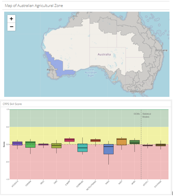
• The Western Wheatbelt AAE (overlaps Western GRDC region) had limited skill for most of the year, with some skill in winter (Figure 2)
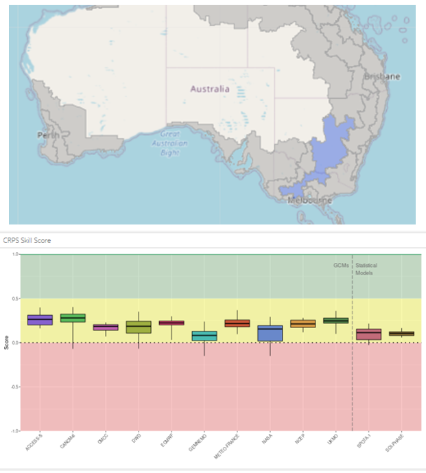
• The skill of forecasts for AAEs overlapping the Southern GRDC region were mixed, with those areas further west (South Australia) having lower skill than areas further east (Figure 3)
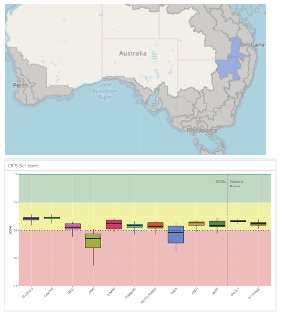
• The Northern GRDC region had higher skill in winter and spring than other wheatbelt AAEs (Figure 4)
• The SCFs based on statistical models (SPOTA-1 and SOI-Phase) did not have superior skill or accuracy to the forecasts based on dynamical models. This included AAEs where the statistical models were originally developed i.e. Queensland/Northern NSW.

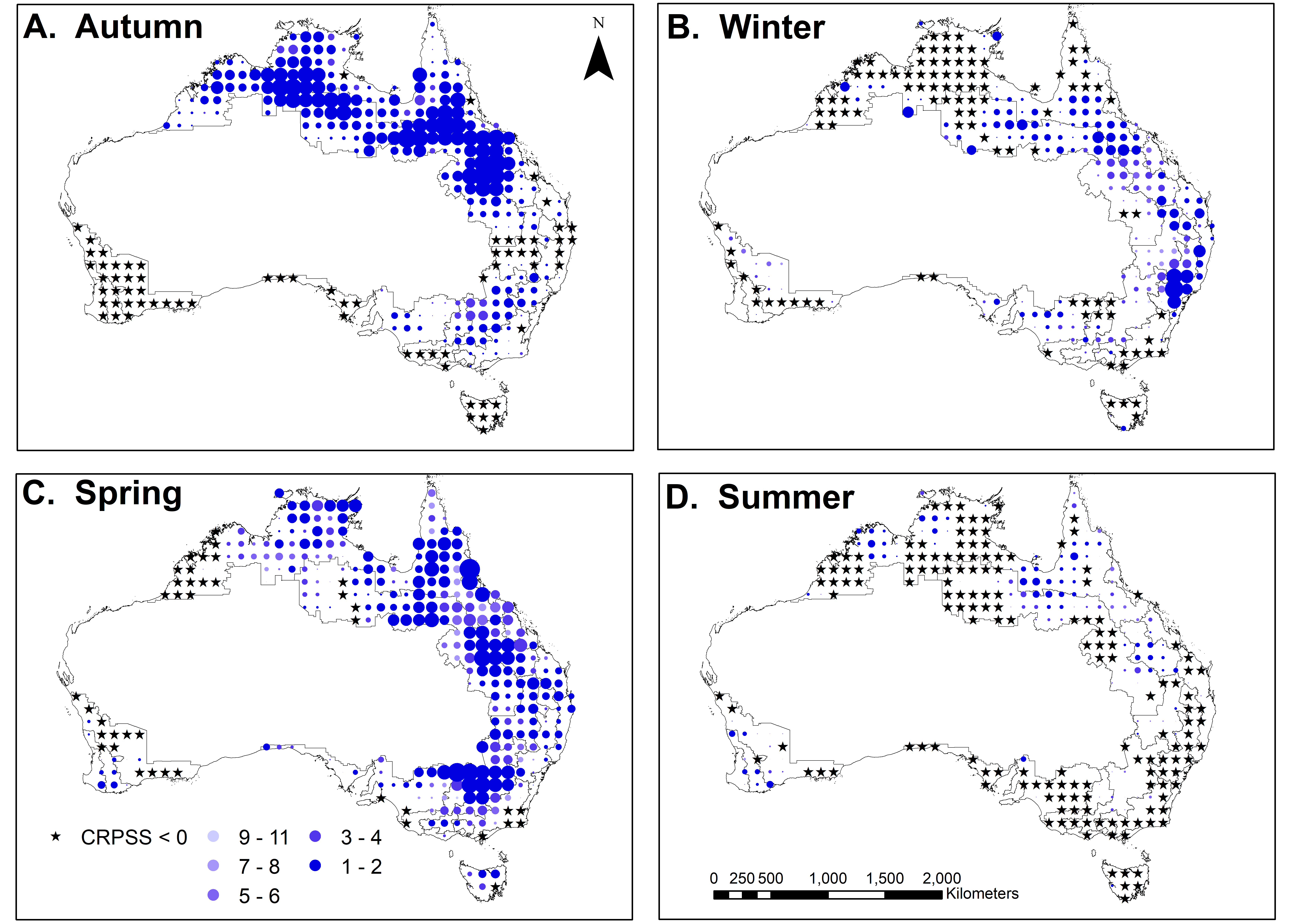Figure 1. The ranking of the Bureau’s model (ACCESS-S1) relative to the other 11 SCFs for a
three-month rainfall forecast window i.e. one meaning ACCESS-S1 is the top-ranking model among the twelve models tested. The ranking was based on the Continuous Rank Probability Skill Score (CRPSS) at that grid point. The size of the symbol is scaled by the CRPSS and values less than zero are denoted by the star symbol (indicating no skill).

Figure 2. Top: Map of Australian Agro Ecological zones, with the Western Wheatbelt of WA in highlight.  Bottom: Continuous Rank Probability Skill Scores (CRPSS) among the 12 SCFs for winter in the western wheatbelt AAE over a three-month forecast period. The background shading of each panel indicates level of skill: red (lower half of graph, CRPSS < 0) – poor or worse than climatology, yellow (middle, CRPSS between 0 and 0.5) – moderate or slightly better than climatology and green (top, CRPSS > 0.5) – good or substantially better than climatology.

Figure 3. Top: Map of Australian Agro Ecological zones, with the Eastern Wheatbelt area in NSW and VIC in highlight.  Bottom: Continuous Rank Probability Skill Scores (CRPSS) among the 12 SCFs for spring in the Eastern Wheatbelt AAE over a three-month forecast period. The background shading of each panel indicates level of skill: red (lower half of graph, CPRSS < 0) – poor or worse than climatology, yellow (middle, CPRSS between 0 and 0.5) – moderate or slightly better than climatology and green (top, CPRSS > 0.5) – good or substantially better than climatology.

Figure 4. Top: Map of Australian Agro Ecological zones, with the Northern Wheatbelt area in NSW and QLD in highlight.  Bottom: CRPSS scores among the 12 SCFs for spring in the Northern Wheatbelt AAE over a 3-month forecast period. The background shading of each panel indicates level of skill: red (lower half of graph, CPRSS < 0) – poor or worse than climatology, yellow (middle, CPRSS between 0 and 0.5) – moderate or slightly better than climatology and green (top, CPRSS > 0.5) – good or substantially better than climatology.

Limitations of the inter-model comparison

The results produced by this study need to be treated with caution. Like all climate inter-model comparisons, the verification process has several caveats that need to be considered when making conclusions from the data. Inconsistencies in hindcast data among forecast systems include differing spatial resolution, hindcast verification periods and ensemble size all contribute to further uncertainties in the analysis. Furthermore, verification of hindcast data does not capture performance of operational forecasts and it is these forecasts that can influence public perception of forecast quality and overall confidence in seasonal climate modelling overall.

Do yield forecasts offer improved performance?

The second part of the project looked at forecasting seasonal patterns in productivity in terms of wheat yield. We used a new software service, AgScore™, developed by CSIRO (Mitchell, 2021). The AgScore service was used to test five different forecast datasets including the Bureau’s ACCESS-S1 and the newly released ACCESS-S2 models as well as the ECMWF-SEAS5 model (European forecasting agency). Three different calibration and downscaling methods were also tested, to compare different approaches applied to the same raw forecast data (ACCESS-S1). These downscaling methods include: a relatively simple quantile-quantile matching approach (QQ) and two more complex approaches - Empirical Copula Post-Processing (ECPP) and Bayesian Joint Probability (BJP).

The AgScore service ingests forecast datasets for a select group of locations and automatically creates and executes workflows that run simulations of wheat and performs verification analyses. The results for a particular forecast dataset are provided to the user as a report card, providing a summary of the performance of the data from an agricultural perspective. The wheat simulations were performed using APSIM and configured in a way to allow for a comparison of a model-based forecast and a climatology forecast. The wheat simulation for a particular location had a fixed sowing date (late April) and used a combination of weather observations and forecasts initiated at different start months (i.e., May, July and September) to grow the crop. This means that a simulation using a forecast data starting in May had a larger contribution of its weather input from the model-based data compared to a forecast starting in September. As in the first component of the study, forecast skill is measured as the level of improvement of the model-based forecast over climatology.

The AgScore service provides a report in the form of an interactive dashboard (Figure 5). The results use several different measures of forecast quality as well as diagnostics to identify underlying issues with the forecasts provided to the service. The target user of the service is researchers interested in climate modelling, development of calibration approaches and agricultural forecasters.

Figure 5. Example of an AgScore™ Wheat report card. Results are presented as an interactive dashboard.

A.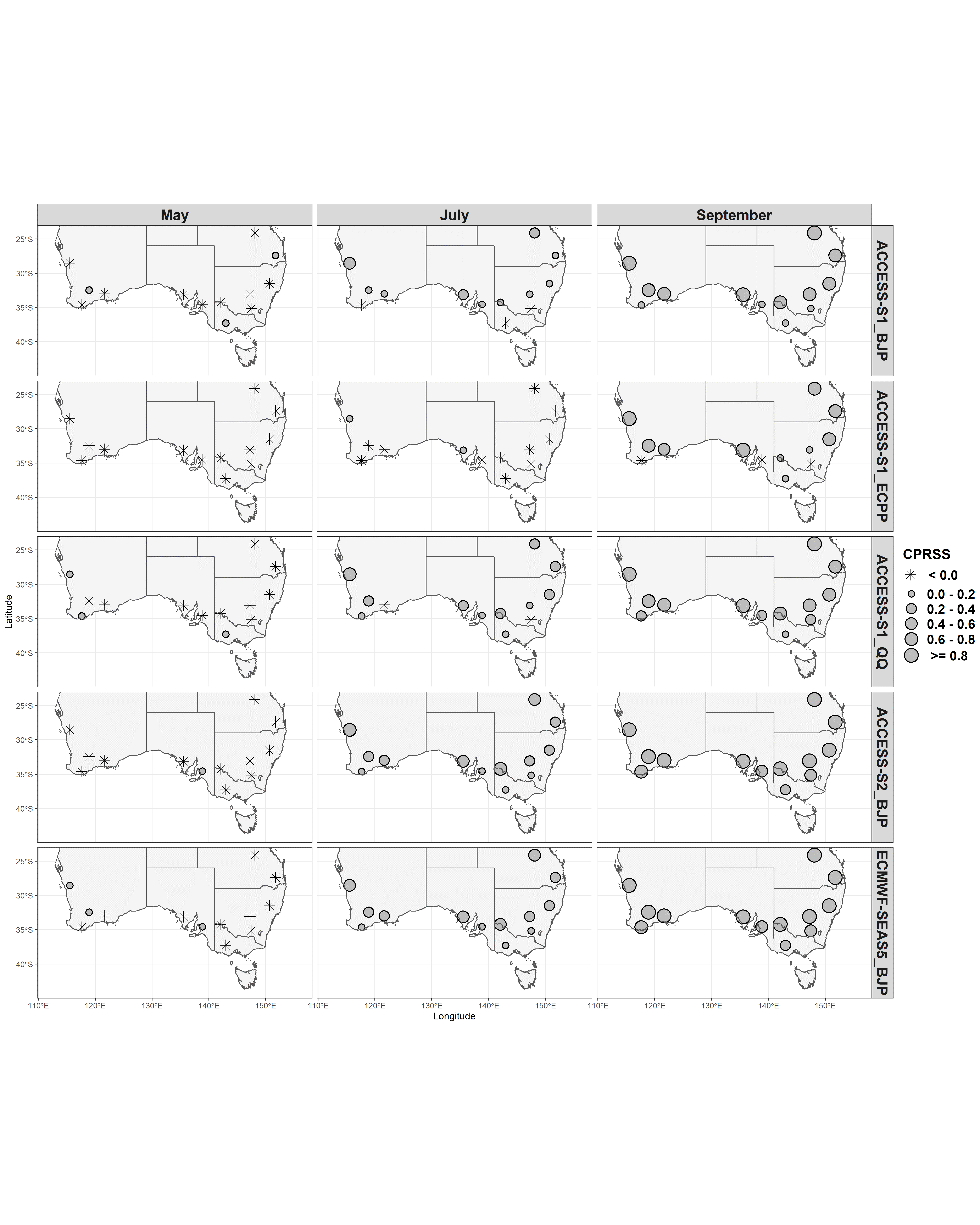

B.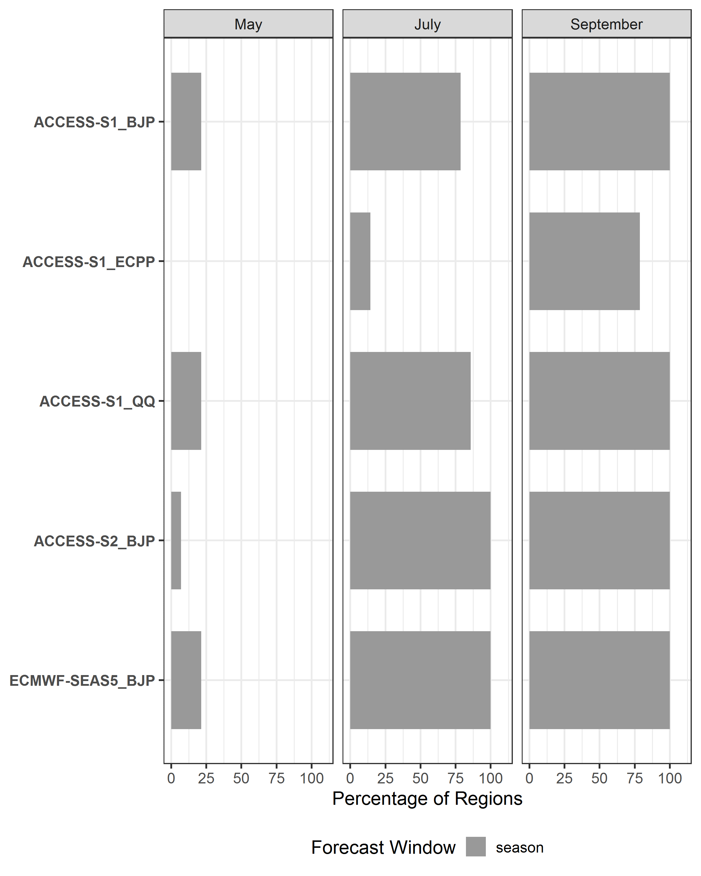

Figure 6A. Map of Continuous Rank Probability Skill Score (CRPSS) for yield among regions for different forecast months and 6B. percentage of regions with a CRPSS greater than 0 (positive skill) for yield across all forecast months. The five different forecasts are denoted by the climate model name and downscaling method (see text for details).,

The key results from this second component were:

• For most locations, yield forecasts based on the Bureau models (ACCESS-S1 and ACCESS-S2) and ECMWF-SEAS5 had skill from mid-way through the growing season (July; Figure 6).
• The new Bureau model (ACCESS-S2) showed small improvements in skill from the previous version (ACCESS-S1; Figure 6 A). This may in part be explained by the former having a longer hindcast dataset (1981-2018) over which to test the performance.
• The downscaling method applied to the climate model data had some influence on the skill of the yield forecasts, with one method (ECPP) having poorer skill compared to the other methods (Figure 6). Whereas no clear differences were found for the other two methods: Quantile Quantile matching (QQ) and Bayesian Joint Probability (BJP). This suggests that some improvements in skill can be realised using the appropriate downscaling method.

Conclusions

While there is a tendency to try and ‘pick winners’ when comparing forecasting performance among different global forecasting systems, this study exposes some of the complexities of taking such a position. We did not identify a single model with superior skill in all locations and seasons. For grains regions there are several models that provide skill for southern and eastern regions during winter and spring. While the Western region has limited skill across the winter growing season, noting we did not include DPIRD’s Statistical Seasonal Forecast system (https://www.agric.wa.gov.au/newsletters/sco), the Bureau’s model, the most widely used seasonal outlook in Australia, ranked highly among the top-performing models.

These results provide a comprehensive and standardised comparison of seasonal forecast systems whilst emphasising the need for improvement in the overall forecast performance. Furthermore, we recommend continued use of the Bureau’s forecast products, but advocate for a consensus-based approach to presenting forecast information. This means presenting results of forecasts from high-performing models’ side-by-side to instil confidence for growers when reading seasonal forecast information.

Forecasts translated into yield-based predictions have obvious benefit to users in that they incorporate multiple climate drivers i.e., rainfall and temperature and integrate seasonal trajectories of plant growth. Our results show that the best forecast systems and corresponding downscaling methods, can provide skill during mid to late stages of the winter wheat growing season (July onwards). This is likely to offer benefit to in-season management decisions around fertilising, marketing and logistics. Both models tested, the Bureau’s new ACCESS-S2 and Europe’s ECMWF-SEAS5 had similar performance and could be applied to existing wheat forecast systems such as CSIRO’s National Graincast™ service (Hochman and Horan, 2019).

References

Centre for International Economics (2014)  Analysis of the benefits of improved seasonal climate forecasting for agriculture, Centre for International Economics, Canberra.

Cowan, T, Stone, R, Wheeler, MC and Griffiths, M (2020) Improving the seasonal prediction of Northern Australian rainfall onset to help with grazing management decisions. Climate Services, 19: 100182.

Duan, W and Wei, C (2013) The ‘spring predictability barrier’ for ENSO predictions and its possible mechanism: results from a fully coupled model. International Journal of Climatology, 33(5): 1280-1292.

Hansen, JW, Potgieter, A and Tippett, MK (2004) Using a general circulation model to forecast regional wheat yields in northeast Australia. Agricultural and Forest Meteorology, 127(1): 77-92.

Hayman, P, Crean J, Mullen, J and Parton, K (2007) How do probabilistic seasonal climate forecasts compare with other innovations that Australian farmers are encouraged to adopt? Aust J Agric Res, 58(10): 975-984.

Hochman, Z and Horan, H (2019) Graincast: near real time wheat yield forecasts for Australian growers and service providers. In: J. Pratley (Editor), Proceedings of the 2019 Agronomy Australia Conference, Wagga Wagga, Australia.

Jagannathan, K, Jones, AD and Kerr, AC (2020) Implications of climate model selection for projections of decision-relevant metrics: A case study of chill hours in California. Climate Services, 18: 100154.

Lacoste, M and Kragt, M (2018) Farmers’ use of weather and forecast information in the Western Australian wheatbelt. Report to the Bureau of Meteorology, Department of Agricultural and Resource Economics, The University of Western Australia, Perth.

Meinke, H, Nelson, R, Kokic, P, Stone, R, Selvaraju, R and  Baethgen, W . (2006) Actionable climate knowledge: from analysis to synthesis. Clim Res, 33(1): 101-110.

Mitchell, PJ (2021) AgScore™: Methodology and User Guidelines, CSIRO, Australia.

Robertson, M, Kirkegaard, J, Rebetzke, G, Llewellyn, R and Wark, T (2016) Prospects for yield improvement in the Australian wheat industry: a perspective. Food and Energy Security, 5(2): 107-122.

Taylor, K  (2021) Producer requirements for weather and seasonal climate forecasting Quantum Market Research, Sydney.

Williams, J, Hook, RA and Hamblin, A (2002) Agro-Ecological Regions of Australia. Methodologies for their derivation and key issues in resource management, CSIRO Land and Water.

Acknowledgements

The research undertaken as part of this project is made possible by the significant contributions of growers through the support of the GRDC, the author would like to thank them for their continued support.

Contact details

Dr Patrick Mitchell
CSIRO Agriculture and Food
Castray Esplanade, Hobart Tasmania 7000
Mobile: 0459 813 793
Email: patrick.mitchell@csiro.au

^TM Trademark

GRDC Project Code: CSP2004-007RTX,