Using common precision ag data layers to accurately and economically ground truth

Take home messages

• Investing in high-quality satellite imagery and analysing crop performance throughout the growing season is key to identifying zones with sub-soil constraints.
• Ground truthing with purposeful soil testing in representative zones is critical for understanding and interpreting the drivers of crop variability. It is important to scrutinise the yield and satellite imagery before investing in soil map layers such as EM38 soil surveys and grid data such as pH maps.
• Management zones, based on ‘yield potential’ are a powerful tool for making seasonal variable rate maps for nitrogen and phosphorus inputs quickly and flexibly.
• The spreading of variable rate soil ameliorants such as gypsum and lime can be carried out precisely and more economically using precision ag map layers, targeting inputs more intensively on the soil types that will respond.
• Creating a ‘precision ag support network’ – including the hardware specialist, the agronomist, analytical map management software or consultant, coupled with the grower’s knowledge, is key to moving forward with precision ag variable management.

Background

Most fields have a degree of inherent soil variability. Soil testing can be a valuable tool to understand the physical and chemical characteristics of variability, however, it may appear to be an expensive and time-consuming process for the grower. Results may seem daunting and complicated to interpret if they’re not collected with a specific focus or goal in mind. It is common for growers to have several years of yield data collected from their grain harvesters. It is less common for growers to be using these data layers to help determine soil zones in a field.

Yield data is valuable when there are several seasons of data in different crop rotations to compare trends. It is even more valuable when coupled with soil survey data and satellite imagery, as these layers can begin to reveal patterns about soil variability changes within a field and how they relate to final yield.

The following case study is designed to demonstrate a process to use data layers to soil test strategically, then show how the results can help make variable management decisions. This process could be replicated in different soil types, using a different base soil layer, not just EM38.

Interpreting yield and satellite imagery to prioritise fields for variable management

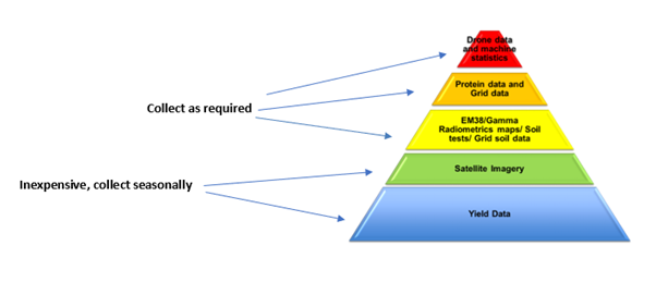
Figure 1. Available precision ag map layers.

There are many precision ag map layers available to the modern grower (Figure 1). The cheapest and most readily available layers, such as yield maps and satellite imagery, give a solid foundation to analyse crop performance before investing in collecting other data layers.

The following is a step-by-step guide for agronomists and growers starting with precision ag data interpretation.

• Pick a field where the cause of the variability is unknown, or less understood.
• The degree of variability can be assessed using the coefficient of variation (or CV%), or standard deviation/mean expressed as a percentage:
  • <= 8% - not very interesting
  • >8% <= 16% worth investigating
  • >16% well worth exploring the cause and pursuing the opportunities.
• Compare yield maps with season rainfall (total and the distribution of the rainfall over the growing season) to remove environmental influence on yield. You are searching for factors within your control to change throughout this process.
• Collect and organise the data layers available to you and ensure they’re accurate (processed).
• Look at cereal rotations and compare the patterns over several different seasons. It is best to omit yield maps that have been heavily impacted by environmental factors such as frost or hail.
• Compare yield maps with in-season imagery:
  • Early season maps are good indicators of topsoil variability
  • Late season maps are good indicators of subsoil variability, as plant roots venture into the sub soil resource.
• Use ‘constant’ map layers to compare with the yield and imagery to begin to find correlations, for example, elevation, EM38 or gamma radiometric data. Grid soil data such as pH may be useful too.
• Develop representative ‘zones’ to test. This may require input and consultation from an agronomist. You are looking for consistent correlations or patterns between maps that are ‘representative’ or ‘typical’ or just simply need more explaining.
• Choose a representative core site in each zone. The aim is to develop a deep and comprehensive understanding of the soil conditions within each zone. Record the latitude and longitude at the soil core site.
• When the cores are taken, (usually to a depth of 90cm), it is best to split the cores by horizons for testing. Take photographs of the cores to help with analysis and track root growth. It is best to take cores throughout spring in a cereal rotation. Consider factors that do not fluctuate quickly here, including soil texture, organic carbon, phosphorus, salt content and pH.
• Use the results to determine overarching soil type for each zone, consider the soil properties at each location, as each zone may require different agronomic management. Also consider the differences down the profile as the crop may experience different growing conditions as the roots move down the profile, which will influence early and late season decisions differently.
• Using the soil core results, make an educated decision on which soil survey data will add value to your farming enterprise. These layers will provide special data across the paddock to help create variable rate management maps. This can be grid sampling or zoned aggregated sampling. Again, consult your agronomist for your individual situation.

A grower case study example – Baroota, South Australia

Farm details

Owners: The Dennis Family
Location: Baroota, Upper North
Average rainfall: 320mm
Crop rotation: wheat, barley, lentil

Method

The case study site to carry out and investigate the strategic coring process was at Baroota, in the Upper North of South Australia. The growers had recently taken over management of the 190ha field and wanted to gain a better insight of the soil constituents. The yield maps were showing variable patterns, and soil variability and past management practices were suspected to be the main drivers.

Paddock performance – evidence of variability

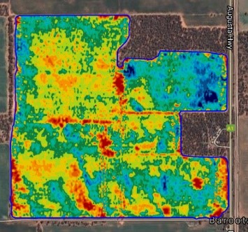
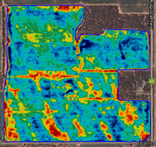
NDVI June 2019                               NDVI Sept 2019                        2019 Barley Yield Map

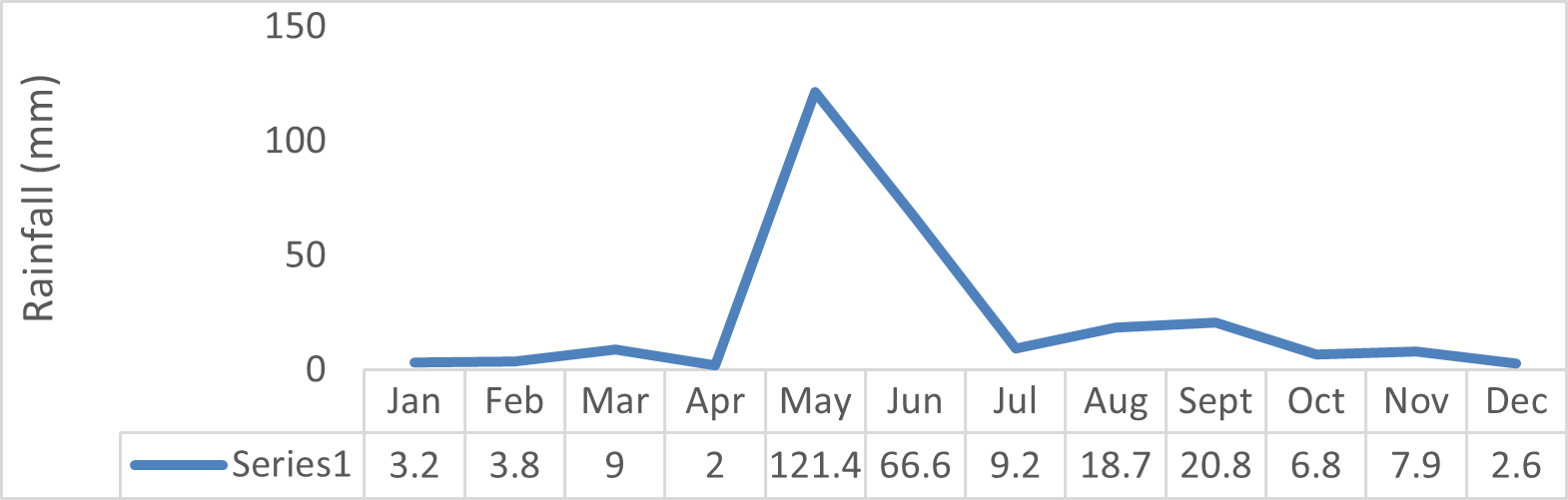
Figure 2. Annual monthly rainfall for Baroota in 2019 (top). Comparing the distribution of rainfall throughout the growing season to satellite imagery throughout the growing season (bottom) can help highlight plant available water (soil texture) and sub soil constraints in the paddock in Baroota.

Adding insight through the addition of a soil survey map and landscape change map

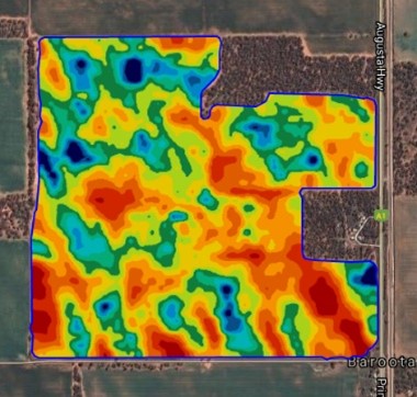
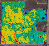
EM38 Soil Survey Map                                                            Landscape Change Map

Figure 3. EM38 soil survey map (left) and landscape change map (right) of the paddock in Baroota.

Local knowledge of the area, grower knowledge, and the yield maps indicated a ‘dune swale’ environment. EM38 soil surveys can be strong indicators of soil texture variability by sensing changes in electrical conductivity in the soil. The landscape change map (processed from data from the seeding machine) supported this theory by highlighting the sandy ‘rises’. The evidence in Figures 2 and 3 led to the decision to use the EM38 map (Figure 4) as a basis for taking strategic cores. Why?

• To determine whether EM38 (electrical conductivity) was in fact a driver of yield variability.
• To understand chemical and physical constraints in these zones which may indicate variable management.

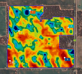
Figure 4. The EM38 Map was chosen as the ‘base layer’ for taking soil cores in representative zones of the Baroota paddock.

Results and discussion

Table 1: Chemical analysis of each of six soil cores taken in the project paddock. Parameters measured include pH, salt content, texture, organic carbon, phosphorus and micro-nutrient deficiencies, and toxicities for each site at dual depths. The chemical driver of this paddock is carbonate (free lime), which influences pH and hence, nutrient availability. The main physical constraint of this paddock is soil texture, hence water holding capacity.

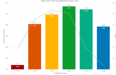
Figure 5. A correlation graph with the Dual EM38 50cm zones vs the yield average within that zone in t/ha.

The above bell curve helps to visually explain the main yield driving factors of this paddock (Figure 5). As electrical conductivity increases, the clay content increases, and so does yield to a point. This can be directly attributed to an increase in plant available water and nutrients. However, there becomes a point where the increased EM38 value brings other limitations into play and yield begins to diminish. In this scenario, this is nutrient toxicity and salinity levels. In the heavier textured soils, leaching of salts and nutrients is reduced and hence, held in the plant root zone creating toxicity issues (blue zones). This correlation helps conclude that the EM38 map is a strong indicator of soil texture and characteristics and is helpful as a template for variable management decisions.

The management decisions and economics

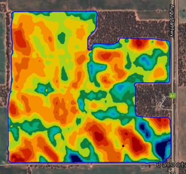
The overarching purpose of strategically coring in different soil zones is to match inputs to the productive capacity of the soil. The EM38 map will be utilised as a template for amelioration and maintenance applications (Figure 6).

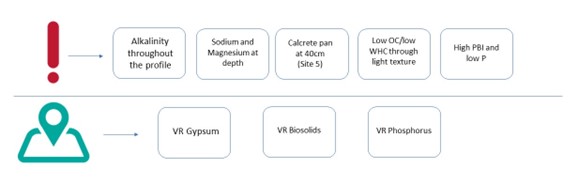
Figure 6. The overarching soil constraints summary (above the line) and the variable rate management options (below the line).

Biosolids/chicken manure variable rate application

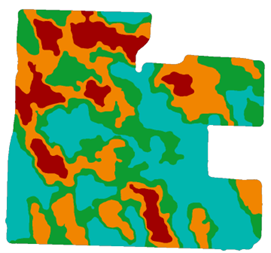
Biosolids is an organic rich amendment which increases organic carbon content of the soil resource, therefore increasing water holding capacity of the soil. The red zones on the EM38 map (low value) will be targeted with a higher rate of biosolids (Figure 7). The upper limit of the biosolids rate will be considered carefully as the product can have high levels of heavy metals which can accumulate within the soil. Additionally, the low rate will also be carefully considered, ensuring that there is enough product to achieve a uniform spread pattern.

Figure 7. The biosolids variable rate prescription map.

Variable rate gypsum application

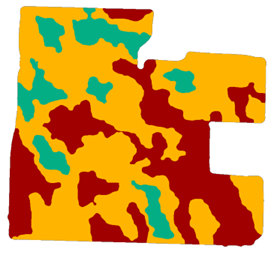
The EM38 map will essentially be ‘inversed’ for a gypsum application, with the higher rates targeted on the blue (high value) zones (Figure 8). Gypsum is recommended in a variable rate application to release sodium from the CEC, allowing it to leach beyond the plant root zone. This will ultimately prevent dispersion and compaction. When sodium is on the cation exchange site of a clay/OC particle, upon wetting the sodium molecules will repel one another, pushing apart soil particles and causing dispersion. Upon drying, this leaves the soil resource ‘structureless’ increasing the required ‘force’ of plant roots to explore the profile and making it difficult to access water and nutrients.

Figure 8. The gypsum variable rate prescription map.

Cost of operation – comparing variable rate with blanket rate

Table 2: Cost of spreading biosolids or gypsum at a blanket or variable rate (A) and the overall cost benefit (B). Area of field: 190ha. Assumption of product sourced from closest supplier to Baroota, working on figures from the grower from past spreading operations.

A

Ref: Agworld

B

Overall cost benefit

This soil profiling process resulted in a net saving of $2,174 through just the gypsum and biosolids spread operations alone. The benefit of future yield improvement through ameliorated soils is not yet realised.

The information from the soil tests is transferrable to other variable management decisions like phosphorus and nitrogen. Most importantly, this field has been profiled for the long term and the chemical and physical limitations are now understood, and can be acted upon and considered in the future.

Conclusion

The value of involving a network of professionals in the process of site-specific precision ag mapping with the purpose of targeting inputs to soil constituents cannot be understated. The grower has a sound understanding of the paddock history through their management, and the areas of their fields that are better yielding will generally be known regardless of what maps they have available.

However, having the maps in a format that is organised allows correlations to be drawn, and makes the maps simpler to interpret, particularly with the addition of site-specific soil tests. This may mean investing in a specialised software package or enlisting the help of a precision ag consultant. The agronomist can assist with interpreting map layers, advise on where to take the soil cores, and help calculate application rates. A machinery dealer can assist with enabling easy flow of data into and out of hardware equipment in the machine. Each of these parties is integral in moving forward with precision ag projects in the business (Figure 9).

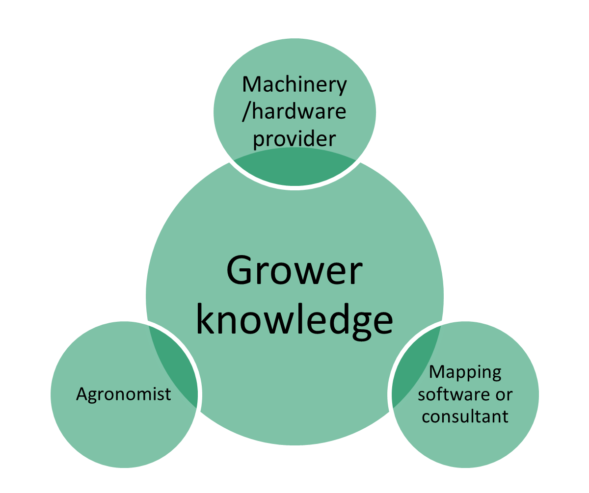
Figure 9. Integration of various knowledge sources optimisessite-specific precision ag mapping.

Acknowledgments

This precision ag case study site was an initiative of Upper North Farming Systems ‘Producer Technology Uptake’ program, Funded by Agrifutures Australia. Thank you to Bethany Humphris, soil agronomist, at Elders Jamestown, for providing agronomic interpretation. Michael Zwar at AgTech Services provided the collection and lab analysis of the soil test data. The map analysis and data processing were carried out by Breezy Hill Precision Ag Services, enabled by PCT AgCloud.

Useful resources

Using precision ag data to accurately and economically soil test

Using precision ag map layers to think about frost differently

GRDC – A profit first approach to precision ag 

Contact details

Jessica Koch
PO BOX 13/51 Koch Road, Booleroo Centre SA 5482
0407 986 557
Jessica.breezyhill@outlook.com
@BreezyHillPAS