Take home messages

• State-of-art modelling allows near real-time estimates of plant available water at spatial resolutions of 20m for the whole-profile.
• A key enabler is 3-D on-farm digital soil maps of soil water holding capacity, which improve the accuracy of PAW estimates by ~10mm.
• 3-D soil maps of constraints allow for better decisions around amelioration and/or input decisions (e.g., fertiliser and fungicides) based on adjustment of seasonal potential yield.

Background

Knowledge of soil variability across a paddock opens up the possibility to manage this variability with the adoption of precision agriculture. Common examples are varying inputs, such as fertiliser, if there are differences in soil type, and therefore seasonal potential yield, or varying ameliorants, such as gypsum and lime, if there are differences in constraints, such as pH and sodicity. This form of precision agriculture is responding to temporally static soil properties but ideally, we would also be able to vary our management according to variation in plant available water (PAW) as it varies across a paddock, and within and between seasons. An extra layer of complexity is that soil varies, not just across a paddock, but also vertically within a profile, and our knowledge of its variability must be three dimensional. Ideally, we would know the vertical distribution of plant available water in the profile and where in the profile our soil is constrained, for example, high sodicity, and how this changes across a paddock.

An ideal future state is that we can map soil properties, such as constraints and water holding capacity, in 3-D across a paddock and, at the same resolution, predict PAW as it changes through the profile and through the season in near real-time in what we call a nowcast of plant available water (PAW).

Over the past decade, a number of enablers have made this a possibility. These include increased computing power and advances in machine learning. Equally important has been the availability of remote sensing products that move beyond NDVI and estimate agronomically useful properties, such as evapo-transpiration (ET) (Guerschman et al. 2022). Furthermore, there have been nationwide efforts to harmonise soil information, with the exemplar in Australia being the soil-landscape grid of Australia (SLGA), which provides baseline 30–90m resolution soil maps for all of Australia (Grundy et al. 2015). These all allow prediction at the within-paddock resolution if they can be brought together in a modelling framework. To this end, the GRDC has invested in two inter-related projects, which are:

• SoilWaterNow: Soil water nowcasting for the grains industry
• Next generation machine learning models for 3-D soil-mapping applications.

In this paper, we illustrate what is possible with one case study farm, and benchmark this when we rely on the SLGA instead of on-farm digital soil maps. More specifically, we present the approach to create the following maps:

• depth to a constraint
• plant available water capacity (PAWC) with and without consideration of constraints
• plant available water.

Method

Study area

The case study is a 975ha portion of a farm in northern NSW where the dominant soil order, based on the Australian Soil Classification, is a Vertosol, which has high clay content. Twenty-five soil cores were taken across the area to a depth of 1m, with each core divided into intervals of 0–15cm, 15–30cm, 30–60cm and 60–100cm, and sent to the laboratory for analysis of a suite of soil properties. In addition, a proximal soil sensing survey was conducted to collect high-resolution apparent soil electrical conductivity (ECa) and gamma radiometrics data. Soil ECa was measured via electromagnetic induction (EMI) using a DUALEM-21S instrument (Dualem Inc., Milton, ON, Canada). Gamma radiometric data were recorded using an RSX-1 gamma radiometric detector with a 4L sodium iodine crystal (Radiation Solutions Inc., Mississauga, ON, Canada). Figure 1 presents examples of outputs from each proximal soil sensor. In general, both respond to soil textural variation, but gamma radiometers respond more to the surface layers and the EMI instruments respond more to subsoil layers. This explains the difference in patterns seen in Figure 1. The smaller ECa values in the northern part of the paddock represent prior stream channels which are common in these landscapes.

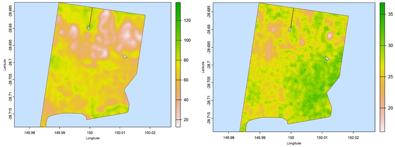Figure 1. Maps of apparent soil electrical conductivity (ECa) 50cm (mS/m) (left) and gamma radiometrics, thorium (ppm) (right).

Mapping soil in 3-D

The focus of the 3-D soil mapping project is to illustrate the use of the machine learning approaches for mapping plant available water capacity and soil constraints, such as pH, sodicity and electrical conductivity (EC). As part of this, we have sampled 75 farms across Australia (Figure 2) using the same sampling process described above.

In a previous GRDC-funded project (UOS2002-002RTX), an approach to map soil in 3-D was developed using machine learning and Gaussian process regression (Wang et al. 2024) that allows the prediction of soil in 3-D at any depth using observations collected from any depth interval. This allows us to not only map soil at the depth at which we are sampling, but any other depth we are interested in. In the example we will present, we show how this capability can be used to map the depth at which a constraint threshold is reached, for example, when an exchangeable sodium percentage (ESP) of 10% is reached. ESP represents a sodicity constraint.

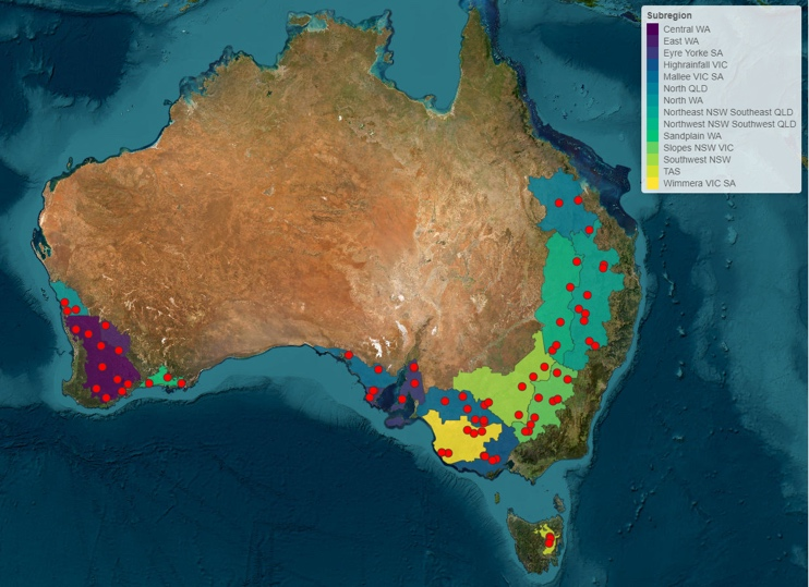
Figure 2. Maps of farms sampled as part of 3-D soil mapping project overlaying grain growing regions of Australia.

In order to estimate plant available water capacity (PAWC), we use what are called pedo-transfer functions (PTFs), where soil properties, such as clay, sand and organic carbon (OC), are used to estimate the drained upper limit (DUL) and the crop lower limit (CLL) using the statistical models. For example:

DUL =  0.2082 + 0.02757OrganicCarbon + 0.002666Clay - 1.73 x 10^-7Sand³.        (1)

PAWC is calculated as the difference between DUL and CLL (DUL – CLL). To map PAWC, we map the inputs such as clay, sand and OC and apply the PTFs on the gridded predictions.

Mapping plant available water (PAW)

Soil water can be predicted by spatially applying a soil water balance equation which is:

ΔS = P - ET - DD - RO         (2)

where ΔS = the change in soil water, P = precipitation, ET = evapo-transpiration, DD = deep drainage and RO = runoff, and all units are in mm. P can be estimated by national rainfall products or on-farm weather stations, ET can be estimated by remote sensing products, DD and RO are mediated by the representation of flow between layers, and the DUL and CLL of individual layers can be estimated by the SLGA or with the on-farm digital soil maps described above.

In the approach presented here, we estimate ET using a 500m MODIS ET (remote sensing) product (Mu et al. 2011) and downscale this to 20m resolution using Sentinel-2 imagery (satellite imagery)  and neural networks. To estimate rainfall, we use the SILO gridded rainfall product (Jeffrey et al. 2001) which is resampled to a paddock average using Thiessen polygons to avoid artefacts caused by its native 5km spatial resolution.

Results and discussion

Mapping in 3-D

Comparison with the SLGA

Figure 3 presents as an example, a map of clay content for the 30–60cm layer using on-farm data and machine learning as compared to the SLGA. Clearly the SLGA does not represent the variability within the paddock and largely missed the large area of prior streams in the northern part of the paddock. The accuracy of the SLGA is 7.8% and the bias (over-prediction) is 4.9% as compared to the on-farm digital soil map.

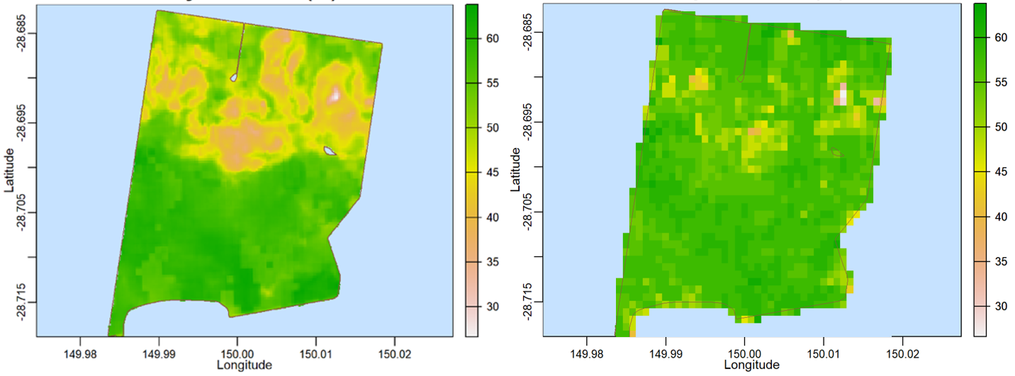Figure 3. Digital soil maps of clay content (%) for 30–60cm using on-farm soil data (left) Soil-Landscape Grid of Australia (right).

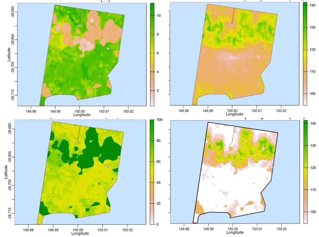
Figure 4. Digital soil maps of ESP (%) for 30–60cm (top-left) PAWC (mm) for 0–1m (top-right) depth to an ESP of 10% (cm) (bottom-left) constrained PAWC (mm) (bottom-right).

Soil constraint mapping

Figure 4 presents maps of ESP for the 30–60cm depth interval (top-left) and a map of depth to an ESP value of 10% (bottom-left), which is a threshold when sodicity may limit root growth and function. The map of ESP for 30–60cm shows that much of the paddock has an ESP of more than 8%, while the prior streams have much smaller values of ~2–3%. The depth to an ESP of 10% was created by mapping ESP at an interval 5cm in the profile and then identifying for each grid location when a value of 10% was reached. The map shows that prior streams do not reach this threshold in the first 1m, but other parts of the paddock reach this typically at depths of 50–80cm.

PAWC mapping

Figure 4 presents maps of PAWC for the whole-profile (0–1m) (top-right) and a constrained PAWC for the whole-profile (0–1m) (bottom-right). The constrained PAWC is created by mapping clay, sand and so on, every 5cm and applying the PTFs to these maps. For each 5cm layer, the PAWC is multiplied by 1 if it is shallower than the depth to constraint threshold, or 0.5 if below this in the profile. This is to represent loss in root function in terms of water uptake when ESP is above 10%.

The PAWC map shows the prior stream part of the paddock has larger values as compared to other parts which have a heavier texture, which means water is bound more tightly, making it less available to plants. The constrained PAWC maps, as expected, shows no change for part of the paddock with no constraints in the profile (the prior streams) and a reduction typically of ~10–20mm in other parts with a constraint in the profile. In this example the constraints are likely to be too deep in the profile to ameliorate but understanding this constraint and PAWC interaction would allow growers to adjust their seasonal potential yield. It should also be noted that the SLGA essentially misses the prior streams (Figure 3) but it does not include constraints such as ESP so a constrained PAWC could not be estimated.

Soil water nowcasting

The water balance modelling framework allows predictions of soil water on a daily time step at the depth intervals that are the same as the digital soil map used to represent DUL and CLL. In the case of the 3-D mapping project, we typically use intervals of 0–15, 15–30, 30–60 and 60–100cm. The water balance equation (Eqn. 1) estimates soil water and we calculate PAW by subtracting the CLL from the estimates. The model generates a huge amount of data, so we typically focus on one time point and aggregate to the whole-profile (0–1m). But the capability exists to predict at the depth increments that are most useful to growers and agronomists in different soil types and systems.

Figure 5 shows a map of PAW for an example time point (31 August 2024) where all inputs are kept the same, except for the underlying digital soil map used to estimate the DUL and CLL.

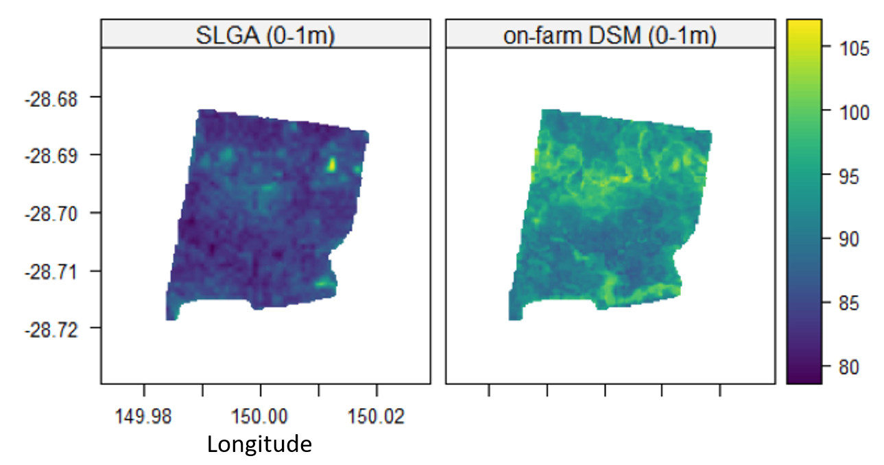
Figure 5. Plant available water (mm) for 0–1m using the SLGA (left) and on-farm digital soil maps (right).

The accuracy of the SLGA is 9.2mm and the bias (under-prediction) is -8.7mm, as compared to on-farm digital soil maps. Similarly to the clay content maps (which are used to estimate the DUL and CLL), using the SLGA results in less variability being represented. Once again, the prior streams are more evident, where in this case, there is more PAW at these locations.

Discussion

Here we found that the SLGA does not represent within-paddock variability and should only be used for paddock-average estimates at best. This is supported by past work by Han et al. (2022). The accuracy of the PAW estimates using the SLGA was 9.2mm, which, if we assume a water-use-efficiency of 22kg wheat grain yield per mm water, translates to an error of 0.20t/ha, if using this information for making a decision about seasonal yield potential for this point in time, with errors expected to accumulate over a season. This is ignoring any constraints which are evident in this example, which, if considered, would be expected to improve the estimate of seasonal potential yield. The underlying digital soil maps could also be used to guide variable-rate application of soil amendments, and the application of strategic tillage in some parts of the paddock but not others based on where it’s needed.

In terms of costs, the sampling and laboratory analysis were undertaken by commercial providers and cost approximately $12 000 and preliminary results indicate that the sample number of 25 cores is sufficient up to ~1 500ha. Work is well progressed with project partner PCT AgCloud to enable growers and/or consultants to generate these maps using their software with an example screenshot shown in Figure 6 where a map of exchangeable sodium has been created with EMI and gamma radiometrics data.

It is beyond the scope of this paper to present, but we are currently repeating what is presented here for all 75 farms (Figure 2) sampled as part of the 3-D soil mapping project. This will give a regional-specific understanding of the quality of the predictions of on-farm digital soil maps as compared to the SLGA. The analysis will also be used to develop better sample size guidelines. This will allow growers to have a better idea about the value proposition of investing in this data collection. The results for all 75 farms will be presented in a future Groundcover article.

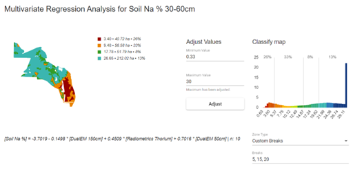
Figure 6. Screenshot of prototype implementation in PCT AgCloud.

Conclusion

State-of-art modelling allows estimates of PAW for any dryland paddock in Australia, leveraging off national and global soil, weather and remote-sensing datasets. These are, at best, useful for estimating paddock-average PAW, but investment in the creation of on-farm digital soil maps allows for estimates of PAW as it varies across a paddock. This information – especially when delivered in a user friendly format through a commercial partner - could help growers and agronomists with many agronomic decisions such as what depth to sow at to chase moisture, what mid-season nitrogen rate to apply based on updated assessments of yield potential, how well a crop is likely to withstand an upcoming heat wave based, etc.  The same on-farm digital soil maps can be used to guide the variable-rate application of soil amendments, and planning on what areas within a paddock would benefit from strategic tillage, and which wouldn’t.

Acknowledgements

The research undertaken as part of this project is made possible by the significant contributions of growers through both trial cooperation and the support of the GRDC, the authors would like to thank them for their continued support. We are also thankful to our industry partner Precision Cropping Technology for who we have leveraged off their extensive network of clients and who are providing a path to market for this research.

References

Grundy MJ, Viscarra Rossel RA, Searle RD, Wilson PL, Chen C, Gregory LJ (2015) Soil and landscape grid of Australia. Soil Research 53(8), 835–844.

Guerschman JP, McVicar TR, Vleeshower J, Van Niel TG, Peña-Arancibia JL, Chen Y (2022) Estimating actual evapotranspiration at field-to-continent scales by calibrating the CMRSET algorithm with MODIS, VIIRS, Landsat and Sentinel-2 data. Journal of Hydrology 605, 127318.

Han SY, Filippi P, Singh K, Whelan BM, Bishop TFA (2022) Assessment of global, national and regional‐level digital soil mapping products at different spatial supports. European Journal of Soil Science 73(5), e13300.

Jeffrey SJ, Carter JO, Moodie KB, Beswick AR (2001) Using spatial interpolation to construct a comprehensive archive of Australian climate data. Environmental Modelling and Software 16(4), 309–330.

Mu Q, Zhao M, Running SW (2011) Improvements to a MODIS global terrestrial evapotranspiration algorithm. Remote Sensing of Environment 115(8), 1781-1800.

Wang J, Filippi P, Haan S, Pozza L, Whelan B, Bishop TFA (2024) Gaussian process regression for three-dimensional soil mapping over multiple spatial supports. Geoderma 446, 116899.

Contact details

Thomas Bishop
The University of Sydney NSW 2006
0405 023 457
thomas.bishop@sydney.edu.au