Comparing profitability of wheat growing in different productivity districts in SA and the implications for management decision making

Barry Mudge,

Rural Solutions SA

Keywords: cost of production, profitability, decision making

Take Home Messages

• Profitability in lower rainfall areas can still be satisfactory at average yields and is competitive with higher producing regions. However, appropriate business settings are essential.
• Operating mixed farming businesses in low rainfall environments is high risk under current input/output pricing scenarios. These risks need to be managed primarily by maintaining a flexible approach
• Capital gains from land ownership may be poor if productivity gains are poor
• Farmers see advantages in land values being held down by lower productivity levels in allowing them to expand their businesses

Background

Grain production in South Australia occurs over a wide range of climatic zones. This results in wide ranging crop yields with average cereal yields in the more climatically favoured areas ranging up to 4-5 tonne/Ha while more marginal farming country can see average yields down to 1.0 tonne/Ha.

This raises the question of whether the higher yields available to businesses producing wheat in the more favoured regions actually allow these businesses to  produce wheat at a lower cost of production  (COP) (per tonne) than the less favoured areas. Or are there other compensating factors which allow less favoured areas to compete and how does the ratio of the various costs which make up COP vary across different production zones?

It is also of interest to study COP and, more importantly, return on capital for businesses over a range of season types to establish the different risk profiles applicable to businesses operating in a range of production settings. This can be then used to guide managers in establishing critical settings for their businesses to improve long term resilience.

At the same time, productivity of different regions changes over time. Climate change is just one of a number of forces which can drive these changes in productivity.  Technology, variety adaptations, changing input/ output pricing ratios are other potential variations. How, then, does this change in productivity and subsequent adaptation responses reflect in the outcomes for these businesses?

Methodology

Five wheat producing businesses were studied across a production transect varying from highly productive land on Yorke Peninsula (average wheat yield  4.5 tonne/Ha) to marginal cereal growing area in a low rainfall district of the Upper North (average yield 1.3 tonne/Ha). (Note: There are at least two other transects in SA with similar characteristics 1.Eyre Peninsula- Cummins-Lock-Kyancutta-Ceduna  2. Eastern SA- Bordertown-Pinnaroo-Loxton. It is expected that a similar study along these transects would reveal similar results).

All the businesses studied were selected as being of a size sufficient to achieve good economies of scale and were all regarded as being soundly managed using good agronomic practices. Three of the businesses incorporated livestock into their program while the other two were cropping only.

The two parameters being studied were the cost of production of wheat and return on total assets employed. These were calculated for a range of season types (very poor, below average, average, above average and very good) using yields and input levels as supplied by the participating farmers. Output pricing and input costs were based on February, 2012 levels.

Qualifications and Assumptions

The majority of the businesses operated land in addition to that owned by the operators (either leased or sharefarmed). For the purpose of this exercise, all land was amalgamated irrespective of ownership. The study focussed on the input requirements for the parcel of land under management (labour requirements, machinery etc) and the profitability of that land parcel but had no interest in who actually received the profits.

In calculating cost of production for wheat, certain assumptions and judgements are required in allocating cost items such as overhead costs to the various enterprises. These will always be subject to interpretation.

The calculated cost of production for wheat included an allowance for capital tied up in land and machinery. Opportunity cost of capital in machinery was included at 10%, while the current market lease value has been used as the return for land.

Results

It is widely recognised that farmers are effectively operating two businesses- in this case, one business is based on wheat growing (and making a profit from that enterprise) and the other business is based on land ownership and is largely concerned with capital growth of the land asset.

1. The business of growing wheat

Given that farmers in the studied regions are almost exclusively aiming their grain output at world markets, their requirement is to keep their cost of production to as low a figure as possible, and hopefully less than what the world market will pay.

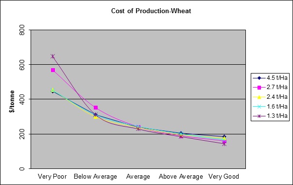
Figure 1. Cost of Production for wheat over different season types for businesses with different average yield expectations

The analysis shows a remarkable consistency in the cost of producing wheat, irrespective of average productivity of the land. COP of wheat at average yields across the various properties varied from $229/ tonne to $244/tonne.

Table 1. Ratio of various cost components of Wheat Cost of Production for different businesses at average yields

The ratio of the various costs showed some significant variations over the production transect. For the highest yielding farm, the proportion of costs attributable to capital return was markedly higher (31%) with this showing generally a decline across the production zones until only representing 17% on the lower yielding farm.

The significance is that the high productivity is being reflected in land value which then demands a financial return. Low yielding country can compensate up to a point by allowing other cost centres to increase (at the expense of capital return) and still keep COP competitive with higher yielding farms. This effectively reflects in a depressed effect on land values. Eventually, however, if yield continues to drop, there is insufficient margin left in the capital allocation and overall COP will rise. In this case, wheat production is unlikely to continue to be profitable (or competitive) and an alternative use for the land tends to occur (eg broad acre grazing).

All the businesses studied showed a profitable outcome at average yields (refer Figure 2- only the highest and lowest yielding farms included). Return on capital across all studied farms varied from 1.4% to 4.8% at average yields and based on 2012 pricing. The analysis shows just how risky it is to operate in the lower producing farming areas. A series of poor years needs to be countered by a rigorous risk management process.

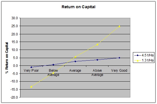
Figure 2. Return on Capital across season types for businesses with different average yield expectations.  

2.    The business of owning land 

Table 2. Estimated Change in productivity and land value of different locations since 1990. 

There have been significant changes in productivity of the study farms over the past 20 years as shown in Table 1.

In general, the higher producing land has increased substantially in productivity, while the lower rainfall land appears to have declined in productivity. Reasons for this are many and are a subject for separate discussion. Importantly though, as shown in the earlier discussion, each of these farms have adjusted to changing circumstances over time and are now operating businesses which are producing wheat at a very similar COP.

• A relatively small climate change induced productivity change is easily overshadowed by other recent changes
• The productivity changes are being captured in land values. The Arthurton farmer has become extremely wealthy just through capital gain. The Willowie farmer’s land has not increased in value. The primary effect of a change in productivity is not on profitability, but on wealth creation (within limits)
• There may be increased opportunity for the lower rainfall farmer to expand, due to affordability of land

Conclusions

Summarising the results

• Profitability in lower rainfall areas can still be satisfactory at average yields and is competitive with higher producing regions
• Operating mixed farming businesses in low rainfall environments is high risk under current input/output pricing scenarios. These risks need to be managed.
• Capital gains from land ownership may be poor if productivity gains remain poor
• Farmers see advantages in land values being held down by lower productivity levels in allowing them to expand their businesses
• Farming systems are very adaptable to change

Implications for business settings

Decisions made in good times are usually the key to survival during difficult periods. Focus on machinery and labour efficiency. Flash paint does not necessarily grow additional crops but timeliness does. Be wary of high debt loads impacting on cost of production.

The current signals for climate change are for a drier and warmer future. If this occurs then this would be expected to adversely impact on crop yields in lower rainfall environments. This suggests that an expansion policy using at least a portion of leased or sharefarmed land may be prudent. Where possible, leases should be flexible based on seasons.

Implications for agronomy practices

Risk management focus is very different between higher and lower yielding regions. In high yielding regions, the focus is firmly on productivity and good agronomy. In the lower yielding regions the risk focus needs to be firmly on methods to limit downside losses in poor seasons without substantially compromising system gains in better years. Flexibility is the key requirement.

The same approach is relevant for individual properties even in lower rainfall districts. Most properties will have areas of inherent high productivity and relatively low risk which consistently outperform other areas on the property. There is a strong argument not to compromise on agronomy in these better areas whilst pursuing a flexible approach in poorer producing country.  

Acknowledgements

This work was completed under a DAFF project studying resilience of mixed farming businesses under climate change.

Contact Details

Barry Mudge

Rural Solutions SA

0417 826790

barry.mudge@sa.gov.au