Optimising performance of current Northern cropping farming systems
Author: Lindsay Bell, Zvi Hochman, Jeremy Whish (CSIRO Agriculture and Food), Andrew Zull (Department of Agriculture and Fisheries Queensland), Peter de Voil (University of Queensland) | Date: 05 Sep 2016
Background
Many cropping systems in the northern grains region are facing substantial sustainability and profitability challenges. Current cropping systems are being challenged by increasing climate variability, declining soil resilience, build-up of soil-borne pathogens such as root lesion nematodes, and increasing reliance on external inputs. The question is: How much more can the productivity of farming systems be improved? To answer this question firstly we need to know about the gap between potential and actual yields on farms. This paper reports on modelling analyses which examine the performance of crops and crop sequences compared to predicted water and nutrient limited potential. A combination of simulation modelling data and regional statistical data shows that many pillar crops are under-performing in the northern region. This identifies that many ‘draggers’ on crop productivity are not related to in-crop management but are associated with the performance of the crop sequence as a whole. Thus, systematic analysis of a range of common crop sequences examined their relative performance in terms of profitability, economic risk and indicators of long-term sustainability.
Yield gaps in the northern region
What is a yield gap?
One promising strategy to increase grain production is to close the gap between yields currently achieved on farms (Ya) and those that can be achieved by using the best adapted crop varieties with the best current crop and land management practices for a given environment (Yw) (van Ittersum et al. 2013).
Water limited yield potential (Yw) is the yield of a rainfed crop when a well-adapted variety is grown with non-limiting nutrients and with biotic stress (weeds, pests, diseases) effectively controlled. Under such management crop growth rate is determined only by solar radiation, temperature, atmospheric CO2, and cultivar attributes such as maturity and the canopy light interception and soil physical attributes (water holding capacity and rooting depth).
Average farmer yield (Ya) is defined as the yield actually achieved in farmers’ fields. To represent variation in time and space in a defined geographical region, it is defined as the average yield (in space and time) achieved by all farmers in the region over a number of years. This number is a compromise between covering seasonal variability and the need to avoid yield trends due to technological or climate change.
The yield gap (Yg) is the difference between Yw and Ya.
Relative yield (Y%= 100 x Ya/Yw) is actual yield expressed as a percentage of water limited yield potential. Is allows for the observation that a 1t/ha yield gap when Ya = 2t/ha is qualitatively different to a 1t/ha yield gap when Ya = 4t/ha.
How is it calculated?
To determine water limited yield potential (Yw) we deployed the APSIM-wheat model (Holzworth et al. 2014) which is well validated for wheat in Australia to simulate wheat grain yields, using 30 years of weather data covering Australia’s grain zone at a median distance apart of 17 km. Three dominant soils were simulated at each weather station area. Sowing rules and nitrogen fertiliser rules were used to ensure that yields were only limited by climate and water conditions. Simulations were run from 1981 to 2010 but only data from 1996 to 2010 were used in the yield gap analysis (Hochman et al. 2016).
Actual annual wheat grain yields obtained by farmers (Ya) was sourced from ABARES at the level of statistical division (SD) annually, and from The Australian Bureau of Statistics (ABS) at the finer scale of statistical local area (SLA) every five years when a census is carried out. The robust correlation between the two data sets was used to estimate Ya at SLA levels in the non-census years.
Each of the values of Ya, Yw, Yg and Y% were then mapped against the 2005 land use map for winter cereals. These maps are available to all through an interactive website.
How large are yield gaps in key crops
Table 1: Yield gap analysis results for Australia and the Northern Region.
| Wheat |
||
|---|---|---|
| Northern Region | National | |
| Actual yield (t/ha) | 1.67 | 1.73 |
| Water-limited yield (t/ha) | 3.61 | 3.45 |
| Yield gap (t/ha) | 1.94 | 1.72 |
| Yield % (=100*Ya/Yw) | 46.2 | 50.3 |
| Exploitable Yield i.e. 0.8 x Yw (t/ha) | 2.89 | 2.76 |
| Exploitable Yield Gap (t/ha) | 1.22 | 1.03 |
| Crop Area (Million ha) | 5.7 | 27.5 |
| Annual Value (Million $) @ $250/t | 1,734 | 7,053 |
Efficiency of current farm crop and crop sequences
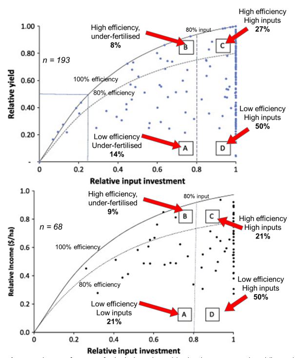
Analysis of farm records from farms across northern NSW and southern Queensland also suggests that there is potential to increase the efficiency of current farming systems (Hochman et al. 2014). A survey of recorded crop yields and inputs over several years was compared with simulations which predicted potential water and nitrogen limited yield in the northern region. This showed that 36 per cent of the crops grown were able to achieve an efficiency of greater than 80 per cent (i.e. actual farm yield compared to potential farm yield for a given input of fertiliser). The yield of a few crops (22%) was limited by low N input relative to their yield potential with over 80 per cent of these crops receiving greater than 80 per cent of the N fertiliser required to optimise their water-limited yield. Fertiliser inputs and sowing time were not shown to be critical factors affecting sub-optimal crop performance, suggesting that other in-crop factors (e.g. disease, weeds and nutrition other than nitrogen) are often reducing crop performance.
However, when the sequences of crops grown in particular fields were simulated this showed even poorer performance with only 29 per cent of fields surveyed achieving 80 per cent of their potential water use efficiency. This suggests that crop sequences in the northern region are less agronomically efficient than the sum of their parts. That is, cropping intensity, the management of fallows and the configuration of crop sequences require closer attention to increase the performance of current farming systems. This also demonstrates that while benchmarks such as crop water-use-efficiency are useful for assessing individual crop performance, it is important that the efficiency of the farming system is evaluated over the full sequence of crops rather than only for individual crops.
Economic efficiency of crop sequences
In response to the above findings, a systematic analysis of common crop sequences used across 10 locations in the northern grains zone aimed to identify any particular crop sequences that were inherently more or less efficient, productive or risky. Analysis captures multiple attributes of the system, including water and nutrient use efficiency, profitability, changes in soil carbon and risks of developing herbicide resistance and root lesion nematode problems. Here we focus on the relative water use efficiency and climate associated risks associated with these crop sequences. It is important to note some limitations of the present analysis. First, the crop sequences simulated were all ‘set’ so that crops were always sown at the end of their sowing window irrespective of soil water triggers being satisfied; this will have increased the likelihood of ‘failed’ crops compared to what might be expected on-farm. Secondly, that the current crop models in APSIM used here don’t capture the effect of extreme heat stress, frost events, or sub-optimal supply of nutrients other than nitrogen. Thirdly, the yields in the crop sequences here are not reduced by losses due to weed competition or from soil-borne pathogens such as crown rot or nematodes; these capabilities are still under development and aim to be included in future analyses. Fourthly, the soils used here had no constraints for crop growth, for example, chickpea which might perform more poorly where subsoil constraints occur. Finally, we have used long-term average prices for each of the crops simulated; risk associated with price fluctuations amongst these are not considered here and the shifts in the relative prices of these crops is likely to shift the relative profitability of sequences.
Methods
A list of the dominant crop sequences applied by growers in each district of the northern region was obtained from focus group meetings with leading farmers and advisers throughout the northern grain production region. Using historical climate data for Dalby and Goondiwindi long-term simulations (110 years) of these cropping sequences were conducted in APSIM, a farming systems model which predicts the production of crops and captures the dynamics of water and nutrients in the farming system. These simulations used rules which ensured each crop in the sequence was sown if a sowing opportunity occurred in their sowing window or at the end of the recommended sowing window, even when moisture levels were marginal. All cereal crops were fertilised to ensure 200kg of N was available at sowing and legumes were not fertilised. All sequences simulated are based on a no-till system with full stubble retention using a common good cropping soil in each district (i.e. PAWC for wheat of 190 mm at Goondiwindi, 193 mm at Trangie and 265 mm at Breeza). Simulations of crop production do not take into consideration losses due to waterlogging, disease, pests, weeds or crop nutrition other than nitrogen.
Gross margin (GM) analysis was conducted over each of these sequences using the equation below. The baseline variable cost for each crop included in-crop pesticide applications, planting and harvesting costs but did not include inputs of N fertiliser and fallow spray frequency as these varied amongst the crop sequences. Long-term average grain prices and current variable input costs were used.

Table 2: Assumptions of crop prices and variable costs used in gross margin calculations for crop sequences.
| Crop | Average Price ($/t) (after transport) | Variable costs ($/ha) |
|---|---|---|
| Wheat | 240 | 175 |
| Sorghum | 205 | 218 |
| Chickpea | 400 | 284 |
| Faba Beans | 380 | 341 |
| Mungbean | 550 | 276 |
Economic efficiency of common crop sequences
In order to compare the relative performance of various crop sequences involving a range of crops over differing periods, the economic efficiency of crop sequences was calculated as the gross margin return per hectare per mm of rain. Like crop water-use-efficiency this enables various production systems to be compared in terms of their efficiency of converting available rainfall into earnings rather than just yield. This approach provides a useful benchmark for establishing an achievable economic efficiency in different production environments and clearly demonstrates that this varies across environments.
This analysis showed that the worst performing crop sequence ranged from 12-35 per cent less economically efficient than the best crop sequence. Differences amongst crop sequences in their economic efficiency were small at Goondiwindi, Narrabri, Mungundi and Coonamble, but larger at Breeza and Trangie. A wheat-wheat-chickpea rotation had the highest economic efficiency at all locations in northern NSW; bearing in mind the analysis did not account for losses due to pathogens or weeds. However, the long-term sustainability of this rotation is questionable as it had the highest risk of accumulating root lesion nematodes and the highest risk of developing herbicide resistance.
Table 3: Mean simulated economic efficiency ($ GM/ha/mm rain) for a selection of prevailing crop sequences at six locations in northern NSW.
| Crop seq.# | SChxWxx | SxSxSChxWxx | SxSxSxxChxWxx | SxSxSxxWMgx | SxxChxWxFbxWxx | SxxChxWxx | SxxWxChxWxx | xWxxxChxx | xWxChxWMgx | xWxWxCh | xWxWxCa | xWxca | xWxCHxWxCa | Range | %variation (range/max) |
|---|---|---|---|---|---|---|---|---|---|---|---|---|---|---|---|
| Locations | |||||||||||||||
| Goondiwindi | 0.47 | 0.45 | 0.44 | 0.47 | 0.50 | 0.06 | 12 | ||||||||
| Mungundi | 0.38 | 0.38 | 0.40 | 0.35 | 0.40 | 0.41 | 0.06 | 15 | |||||||
| Narrabri | 0.44 | 0.41 | 0.44 | 0.45 | 0.52 | 0.49 | 0.11 | 21 | |||||||
| Breeza | 0.80 | 0.74 | 0.65 | 0.66 | 0.81 | 0.94 | 0.29 | 31 | |||||||
| Coonamble | 0.47 | 0.58 | 0.60 | 0.69 | 0.69 | 0.12 | 17 | ||||||||
| Trangie | 0.69 | 0.71 | 0.83 | 0.68 | 0.63 | 0.80 | 0.30 | ||||||||
# - x = fallow; S = sorghum; W = wheat; Ch = chickpea; Ca = canola; Fb = Fababean
It was rare that a particular sequence was more favourable across the full range of climatic conditions (Figure 2). For example, at Goondiwindi in 50 per cent of years the wheat-wheat-chickpea system had the highest economic efficiency but other crop sequences were higher in the other 50 per cent of years. Similarly, in favourable seasons, sequences involving double crops performed best, while under less favourable conditions they performed worst. Systems with long fallow periods to transition from winter to summer crop performed better in the less favourable years, but because they have lower crop intensity (i.e. less crops per year), they were less able to capture opportunities in more favourable conditions. This suggests that further examination of how crop sequences could be tactically adjusted in response to seasonal conditions could identify options which both capture upside opportunities and minimise downside risks.
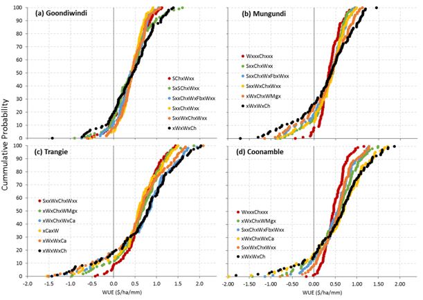
Figure 2: Cumulative probability of economic efficiency (i.e. weighted annual gross margin/mm rainfall) simulated over 110 years for six common crop sequences at (a) Goondiwindi, (b) Trangie, and (c) Breeza.
Risk-return of various crop sequences
The amount of rainfall transpired by crops, or conversely the proportion to time in fallow, were found to be critical drivers of economic efficiency (i.e. the average annual GM over the full crop sequence) and downside risk (i.e. the gross margin in the worst 20% of years). Figure 3 shows the different relationships at four locations between average sequence gross margin and proportion of time in fallow for the full set of crop sequences. At Goondiwindi, Trangie and Coonamble, there is a clear decrease in average sequence gross margin as the proportion of time in fallow increase, while at Mungundi, a higher risk and more marginal environment, this relationship was flat indicating a wide range of fallow frequencies could result in equivalent average sequence gross margins. On the other hand, downside risk (i.e. lower GM in worst years) was decreased as fallow frequency increased, though this relationship was weak at Goondiwindi. This clearly demonstrates the trade-off between increasing potential returns and managing risk across crop sequences.
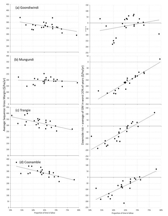
Figure 3: Relationship between time in fallow and gross margin on average of all years (left) and in the worst 20 per cent of years (right) at (a) Goondiwindi, (b) Mungundi, (c) Trangie and (d) Coonamble across a range of 22 crop sequences currently used across the northern grains region.
Crop sequences also varied substantially in their balance of risk and return (Figure 3), and sequences shifted in their relative performance at different locations. Figure 3 plots the average gross margin return of a crop sequence against the proportion of crops grown in that sequence that failed to make a positive return for a full range of 22 crop sequences that are operated commonly in the northern grains region; lines indicate the median of these 22 sequences and delineate the relative performance of crop sequences in terms of high/low risk and high/low returns. This shows that amongst the range of potential sequences there are options that have higher potential yields for a similar level of risk. Typically systems with a greater diversity of crops, and those which utilise a mixture of both summer and winter crops, are those that are more favourable in terms of risk-return.
Sequences with a particularly high frequency of failed crops were those involving a chickpea double crop (e.g. SChxW, SChxWMgx); around 40 per cent and 60 per cent of chickpeas grown as double crops in the sequence did not produce a positive gross margin (data not shown). Crop sequences involving double crops of mungbean, were also risky with about 30 per cent and 40 per cent of these crops failing at Goondiwindi and Mungundi, respectively. At all locations, sequences where the sorghum crops were grown after a short fallow had a higher frequency of failure than those proceeded by a long-fallow (from a previous winter crop).

Figure 4: Mean sequence gross margin (GM, $/ha/yr) vs. frequency of crop failure (i.e. receiving a negative GM) at (a) Goondiwindi, (b) Mungundi, (c) Trangie and (d) Coonamble for 22 crop sequences used throughout the northern grain cropping zone; commonly used crop sequences at each location are shown with hollow symbols.
Useful resources
References
Hochman, Z., Carberry, P.S., Robertson, M.J. Gaydon, D.S., Bell, L.W., McIntosh, P.C., 2013. Prospects for ecological intensification of Australian agriculture. European Journal of Agronomy, 44, 109-123.
Hochman Z, Gobbett DL, Horan H, Navarro Garcia J (2016) Data rich yield gap analysis supports and enriches Global Yield Gap Atlas protocols: a case study of wheat in Australia. Field Crops Research.
Holzworth DP, Huth NI, Devoil PG et al. (2014) APSIM - Evolution towards a new generation of agricultural systems simulation. Environmental Modelling & Software, 62, 327-350.
Van Ittersum MK, Cassman KG, Grassini P, Wolf J, Tittonell P, Hochman Z (2013) Yield gap analysis with local to global relevance—A review. Field Crops Research, 143, 4-17.
Acknowledgements
The research undertaken as part of this project is made possible by the significant contributions of growers through both trial cooperation and the support of the GRDC, the author would like to thank them for their continued support.
Contact details
Lindsay Bell
203 Tor St, Toowoomba
0409 881 988
Lindsay.Bell@csiro.au
@lindsaywbell
Was this page helpful?
YOUR FEEDBACK