Variable-rate application of grain cropping inputs

Take home messages

• The practical goal of Site-Specific Crop Management (SSCM) is to increase the number of (correct) management decisions per hectare.
• Successful variable-rate application of cropping inputs requires a commitment to understanding the size and cause/s of production variation within fields.
• The potential financial benefits from variable-rate application of cropping inputs varies with each field and farming business, but the potential improvements in gross margin ($/ha) are showing up as significant in both soil ameliorant and crop fertiliser operations.

Background

Site-Specific Crop Management (SSCM) is a form of Precision Agriculture (PA) whereby decisions on resource application and agronomic practices are improved to better match soil and crop requirements as they vary in the field. In practice it creates the opportunity to increase the number of (correct) decisions per hectare made about crop management. It is a logical step in the evolution of agricultural management systems towards increased efficiency of input use in production, minimising waste and improving product provenance.

Variable-rate application (VRA) of cropping inputs is a key component of the suite of differential actions available in the SSCM system (Figure 1).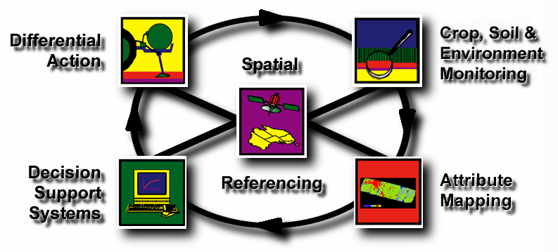

Figure 1: The Site-Specific Crop Management (SSCM) cycle.

Implementing SSCM and variable-rate application of inputs

First it is important that the ‘average’ or uniform agronomy is optimised on a whole-farm basis before SSCM and any need for variable-rate application of inputs is considered. This should ensure whole-farm profitability is currently maximised and allow more accurate and effective determination of if/where/how much variable-rate treatment of input application may be warranted. With this in place, the goal is then to explore opportunities to improve production within each field, which will require:

• The amount and pattern of variability in yield and soil conditions can be measured;
• reasons for the variability can be determined; and
• the agronomic implications of the variability and its causes present a practical opportunity to vary management.

With the understanding that local variability should be seen as the driving factor, it is possible to provide a general strategy to consider for the incorporation of SCCM and variable-rate application of inputs on any farm (Figure 2).

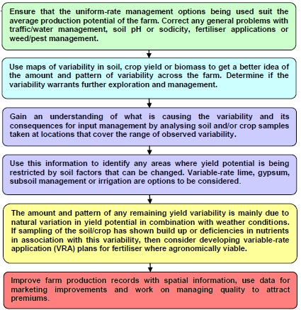
Figure 2: General strategy to drive the incorporation of SCCM and VRA on a farm.

Variable-rate application

The management class concept of soil and crop management is now widely used across Australia, and the introduction of proximal crop reflectance sensor systems has seen the beginning of a shift towards a more fine-scale, whole-field approach to managing production variability. The four main categories of VRA operations can be defined by the scale at which information on variability is gathered/treated and the type of variable-rate technology (VRT) that is used (Table 1). The categories are:

• Map-based management class operations;
• map-based whole field operations;
• real-time management class operations; or
• real-time whole field operations

Map-based management class operations can be undertaken with a wide range of application equipment and applied to any input that is metered onto a field. The main target operations for grain cropping in Australia are:

• Fertiliser;
• soil ameliorants (lime, gypsum);
• pesticides (herbicide, insecticide, fungicide);
• sowing;
• tillage; and
• irrigation.

Real-time, whole field operations need specific hardware to be used for the input being controlled. At present these types of operation are only used to apply nitrogen fertiliser, herbicide and growth regulants.

The potential financial value in VRA using map-based management class operations

Variable-rate ameliorant application

Lime and gypsum application is used to correct soil pH or structural problems respectively. The application rates are usually formulated based on a representative soil analysis result for a whole field. The actual requirement for these ameliorants is usually closely linked to soil type, and where soil type changes within a field, the optimum application rate will usually change. Both these products need to be applied at the correct rates to be effective at improving yield potential.

Identifying the correct rates for different areas within a field using strategic sampling may involve savings in the amount of ameliorant used compared to a blanket-rate application. Where more ameliorant is required than traditionally applied, the cost will be outweighed by the increased effectiveness of the treatment to improve yield potential. The specific financial benefits will depend on the variability in soil type and previous management practices on every farm.

Figure 3 shows a soil apparent electrical conductivity ( EC_a) map (a) and the subsequent classification of the field into two potential management classes (b). Sampling for soil pH within these classes produced the results in Table 2, with 83 per cent of the field requiring no lime application. If the field had not been sampled by management class, and soil from Class 1 used to represent the whole field, then this saving would have been lost. If soil from Class 2 was used to represent the field, then no lime would have been applied and a potentially significant yield loss in Class 1 may have occurred in this and future seasons.

Table 1: The four categories for VRA of nutrient operations are defined by the scale at which information on variability is gathered and the category of VRT equipment.

	Management class treatment of variation	Whole field treatment of variation
Map-based	A map of broad areas where different management is required is used to describe where rate changes will occur. Examples: Nitrogen applied at three different rates to three management classes. Lime only applied in areas previously identified as requiring pH adjustment.	A map of variability across a whole field is used to determine continuous rate changes. Examples: Phosphorus applied based on the pattern of removal from previous yield map/s. Pre-emergent herbicides applied based on a map of soil organic matter content.
Real-time	A map of broad areas where different management is required is used to describe where base rates will change. Real-time sensors are then used to measure variability within each management class and vary application around the base rates. Examples: Base nitrogen rates are calculated for each of three classes. A crop reflectance sensor is then used during application to measure variability in crop condition within each class and vary application up or down from the base rate. Maps of areas where broad-spectrum herbicide is to be applied are combined with reflectance sensors to deliver specific action chemicals to detected weeds.	Variability across the whole field is sensed and used to control treatment rates during application. Examples: Only green weeds, which are detected in fallow using reflectance sensors, are treated with herbicide. Crop reflectance sensors are used to control nitrogen application rate variation around a single base rate.

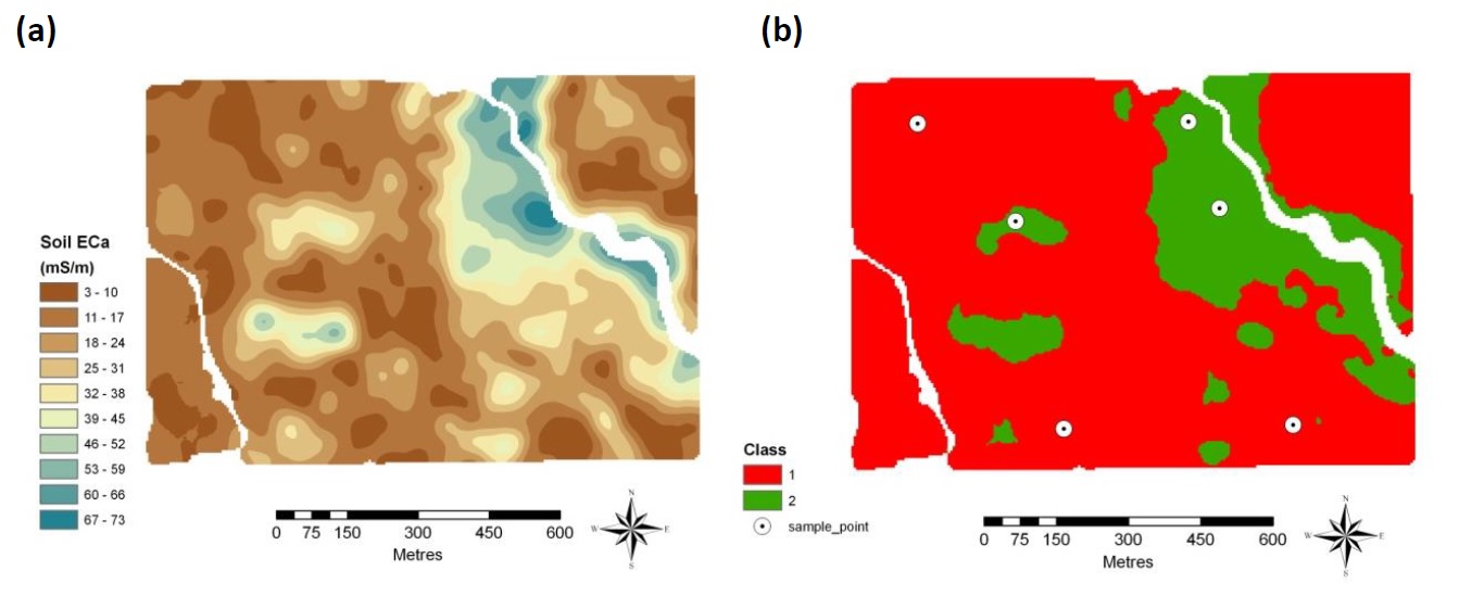
Figure 3: Soil EC_a map (a) and a potential management class map (b) used for soil pH sampling.

Table 2: Soil pH results, lime recommendations and treatment costs for the field in Figure 3.

Field portion	Size (ha)	Topsoil pH	Lime recommended (t/ha)	Cost @ A$50/t spread (A$/area)	Cost of whole field treatment at pH 4.8 (A4/area)
Class 1	16	4.8	1.3	1040	1040
Class 2	79	5.7	monitor	0	3710
Total	95	-		1040	4750

Variable-rate nutrient application

The potential financial benefits associated with variable-rate fertiliser application are also specific to each farm and field. The value of variable-rate fertiliser application will depend on the amount of variation in soil type, landscape, inherent nutrient reserves within a field and the prices for fertiliser and crop product. The suitability of the previous uniform-rate applications and the fertiliser timing strategy (e.g. all up-front, the use of split applications and whether both up-front and split applications are variable-rate) will also affect the size of financial benefit that may be achieved.

Figure 4 shows the fertiliser prescription and application maps along with the subsequent yield for a nitrogen response trial established in a 79ha field divided into two potential management classes. The whole-field average application rate for the paddock was 60kg N/ha.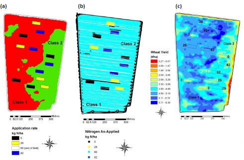

Figure 4: (a) The management class map with VRA trial prescription (b) the as-applied map for a nitrogen response experiment. Uniform field treatment was 60 kg N/ha. (c) the wheat yield map.

The season was above average in rainfall with growing season rain (June-November) of 350mm, or in the 70th centile. To identify the optimum application rate from the trial, the yield response functions for the two classes using the average yield data from the strips were compiled (Figure 5a). Marginal rate analysis (marginal revenue=marginal cost) (Figure 5b) using prices for the season shows that the optimum rates of applied nitrogen fertiliser were 109kg N/ha and 39 kg N/ha for Class 1 and 2 respectively.

With this information, it is possible to compare the gross margin (GM) under standard management to the GM achievable under optimum-rate management. The GM is calculated by multiplying the yield by price and deducting the cost for the quantity of fertiliser applied. Where the GM of the standard management is less than the GM of optimum-rate management, the difference is termed a ‘net wastage’ of standard management. In the opposite scenario the difference would be a ‘net gain’ for standard management.

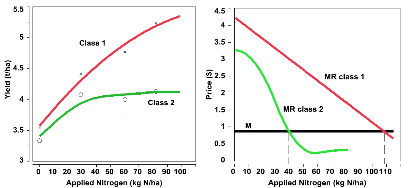
Figure 5. (a) Yield response to applied nitrogen fertiliser from the trial in Figure 2. Uniform field = 60 kg N/ha. (b) MC=MR analysis shows Class 1 optimum = 109kg N/ha; Class 2 optimum = 39 kg N/ha.

Two simple management response scenarios can be considered here to make use of this information on variability. Scenario one would maintain the total amount of fertiliser applied to the paddock but moves the over-application on Class 2 to Class 1. This would keep fertiliser costs constant and result in yield gains in Class 1 that would improve the gross margin by $11.50/ha across the field. Scenario two would aim to apply the optimum amount to each Class, requiring an additional 1.4 t of nitrogen to achieve the yield goals of 5.4 t/ha in Class 1 and 4.0 t/ha in Class 2. However the increased yield would mean that the gross margin for the paddock would be improved by $25/ha.

These figures are a function of fertiliser costs and crop prices obtained in the specific year of each trial. To provide a simple way of standardising the wastage figures between the years, the total net wastage can be compared to the total fertiliser bill for the individual field average application in that year. This provides an estimate of the wastage as a proportion of the fertiliser input costs, i.e. the investment in fertiliser each year. It is calculated as a ratio:

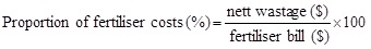(Eq. 1)

In this example the proportion of fertiliser costs that are potentially being wasted using standard management are 22 per cent and 45 per cent for scenarios one and two respectively. The results of a further 18 phosphorus (Table 3) and 15 nitrogen (Table 4) trials across Australia show a median value of 99 per cent for phosphorus and 97 per cent for nitrogen, suggesting that the potential financial benefit to be gained over a number of seasons by knowing more about the optimum rates of fertiliser for a field could be conservatively equal to the amount of money traditionally outlaid on fertiliser. For example, if the average phosphorus inputs were $40/ha/year, then improvements in gross margin of the same amount per year may be possible.

Obviously the seasons do impact on the yield results and the gross margin. It is also important to understand that these optimum fertiliser rates have been determined at the end of the season. However these figures do show that there are worthwhile financial gains to be made by exploring improvements in the efficiency of fertiliser use.

Table 3: Results of gross margin analysis comparisons between field average application of phosphorus fertiliser and that possible under optimum rate management (18 experiments).

Value	Minimum	Median	Maximum
Field size (ha)	34	43	110
Crop Yield (t/ha)	0.5	1.7	5.6
Net wastage ($/ha)	8	48	103
Proportion of seasonal N fertiliser costs (%)	30	99	236

Table 4: Results of gross margin analysis comparisons between field average application of nitrogen fertiliser and that possible under optimum rate management (15 experiments).

Value	Minimum	Median	Maximum
Field size (ha)	22	79	130
Crop Yield (t/ha)	0.4	2.5	4.9
Net wastage ($/ha)	4	39	103
Proportion of seasonal N fertiliser costs (%)	12	97	372

Conclusions

The tools for variable-rate management of agricultural inputs combine a variety of hardware, software and operational techniques. The usefulness of each tool can vary from site to site, and it is becoming more evident that the best information for VRA management can be gathered from within the boundaries of each field. The present systems that are being researched and employed in Australia are not designed to, or capable of at present, totally replacing industry professionals and farmers in management decisions. However they do provide information, and the means, to improve input use-efficiency. The potential financial and associated environmental and risk management benefits appear significant and should impact all sectors of the industry and the wider community.

Contact details

Brett Whelan
Precision Agriculture Laboratory,
The University of Sydney,
1 Central Avenue,
Australian Technology Park,
Eveleigh, NSW, 2015
02 86271132
brett.whelan@sydney.edu.au