Risk and enterprise mix

Take home messages

• Managing risk is not about the middle or the average, it is the opposite. It is appreciating what happens at the extremes, the size or value of these extremes and how often they occur.
• Understanding the probability of different yield and price values occurring and if these values are correlated is essential in understanding risk.
• Usually diversification reduces risk (both downside but also upside risk).

Introduction

Risk is a natural and accepted part of farming. Australian agricultural production (based on value of output) is the most volatile in the world and the most volatile sector of the Australian economy (Keogh, 2013). This volatility conveys a level of risk that needs to be managed. Given most farmers are still operating despite two centuries of volatility, this suggests that they have developed long term strategies and operational tactics to cope with this ongoing challenge.

There are many strategies farmers use to manage production risk. Diversification in crop and pasture type, enterprise mix, targeting multiple markets and property location are common strategies. So is managing input costs, especially when production and prices can be highly variable.

Understanding risk

When we talk about risk most of us immediately think about the negative consequences if an action goes bad. Dictionary definitions re-inforce this thinking. However this is only one aspect of risk. The word risk is derived from the Italian word risicare, which means 'to dare'. To manage risk effectively we need to understand both the downside (the potential harm from taking a risk) and also the upside (the opportunities that taking a risk can offer).

There is no reward without risk. In farming, risk is a necessary part of making returns. Managing risk is about making decisions that trade some level of acceptable risk for some level of acceptable return for an acceptable amount of effort. Decisions can be made to reduce risk, but it usually comes at a price, namely lower returns.

A common definition of risk is likelihood by consequence. In other words risk requires knowing how often an event happens (the frequency) and what is the impact (the value) when it does happen. A decision that increases risk will either increase the likelihood of an event happening and/or increase the consequence if it does occur. This increased consequence may be a greater return, not just a greater loss.

We must remember everyone has a different position on risk. Financial security, stage of life, health, family circumstances and business and personal goals can all influence the amount of risk an individual is willing to take on. This position can change rapidly, sometime triggered by sudden events. Importantly no position is right or wrong, it is what the individual is comfortable living with.

Average values are commonly used in agricultural extension. We present average yields, average prices and average costs. While these averages convey a value (and are convenient), they rarely present the frequency of this average occurring. This would be fine if we consistently got these average values, but in agriculture we rarely do. The key drivers of profit in agriculture, namely yield, prices and some costs have a range of values within and between production periods. If we use averages for analysis, it usually over estimates the profits and hides the volatility in those profits (Nicholson, 2013).

Managing risk is not about the middle or the average, it is the opposite. It is appreciating what happens at the extremes, the size or value of these extremes and how often they occur.

Analysing risk

As described previously the derivation of risk is 'to dare'. This implies there is opportunity but it also implies a choice. As individuals we can influence how much risk we expose ourselves to by making choices.

Insights from the Grain and Graze program would suggest farmers mainly inform their decisions around risk, based on past experience and intuition or instinct. Doing the ‘sums’ to understand the likelihood and consequence is much less common.

Through the Grain and Graze program we have developed a relatively simple way to put some numbers around the risk in a farming business. It is based on Excel with an additional program called @Risk (Palisade website). Firstly the risky variables in a business are identified. These are inputs that we have little or no control over at the start of the season and are typically yields, prices and some costs. Graphs are created that show the amount or value of this risk and how often this amount or value occurs. It includes extreme and more common results and is referred to as distributions or frequency histograms. The broader the range in values, the greater the volatility or risk (Figure 1).

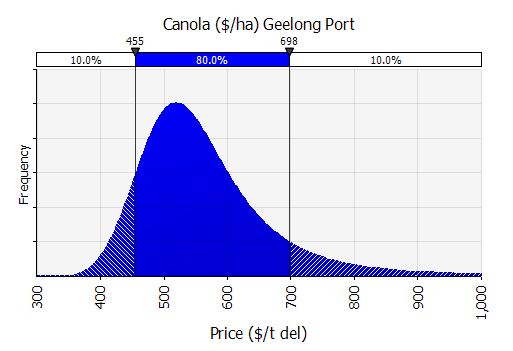
Figure 1. Example of the frequency of weekly prices for canola at Geelong port from 1 July 2003 to 30 June 2016, inflated to June 2016 values. (Ag Commodity Prices - Grain and Graze3 website)

These ‘risky’ distributions are then substituted for the average values used in calculations. For example we may have used an average price for canola delivered at Geelong of $567/t. By substituting this distribution, the program will do some calculations with a price around $567/t, but will also do calculations with prices at $450/t, $500/t, $600/t and even $800/t. However the frequency these prices occur will be different. There will be more calculations around $500/t than around $450/t or $600/t and many more than around $800/t.

The same can be done for yields (and some costs, although most costs increase in price but are not highly variable throughout the season). When the risky yield, price and cost values are combined; they reflect what happens in real life. For example we may have a high yield but poor prices, so our gross income is about average. Less often we will have poor yields and poor prices and conversely we occasionally get high yields and high prices. Adjustments can also be made to link events such as often getting higher prices when yields are poor.

We create these distributions through a combination of historic information (‘form guides’) and gut feel. I call this ‘framing the odds’. Each distribution can be customised to suit your location, soil type, frost risk, etc.

Not all risks are equal. The computer program enables a comparison between the risky variables. For example, we might have a farm with 20 or so distributions but not all of these risks are of equal influence to our final profit. Some create more volatility than others and some are more influential in making or losing large amounts of money. We can identify these and examine the impact because we are able to change them. This scenario analysis is extremely valuable as it enables an understanding of the risk implications of large (and small) changes on the farming business before we make the changes.

Correlations

One reason for diversifying enterprises is to ‘decouple’ price and yield movements. We grow different commodities so if one fails to produce, a different crop or enterprise may still produce something. How strongly yields and prices are linked are referred to as correlations.

Correlations (co- meaning ‘together’ + relation) can be calculated mathematically. The numeric scale used for correlations is 0 to ±1 and is commonly referred to as the ‘r’ value (or correlation co-efficient). If there is no connection or dependence between two variables then it is considered a zero (0) correlation. If one variable exactly follows the size and direction of the fluctuations of the other it is positively correlated and given a value of one (+1). Conversely, if one variable exactly follows the size and direction of the fluctuations of the other, but in opposite direction, it is negatively correlated and given a value of one (-1).

The r value can be broadly classified into ‘strengths’:

• Strong with r greater than ±0.8.
• Medium with an r value between ±0.5 and ±0.8.
• Weak with an r value less than ±0.5.
• None with an r value of 0.

Knowing a weak r value can be just as useful as knowing a strong r value because the weakness implies that there is no connection between the two variables, so they should be considered independent of each other.

Price correlations for common crops and livestock enterprises are provided (Tables 1 and 2).

Table 1. Correlation between common crops (July 2003 to June 2016).

Table 2. Correlation between sheep enterprises (July 2003 to June 2016).

Correlations can also be easily created between enterprises (Ag Commodity Prices - Grain and Graze3 website).

Enterprise mix

Changing the enterprise mix, both in the type and scale of these enterprises changes the risk profile of a business. The following example is for a 920 ha farm near Colac in Victoria, but is based on a real farm. The key values are:

• 250 ha ‘good’ cropping country, 250 ha of ‘marginal’ cropping country (flat and gets very wet).
• ‘Good’ cropping country rotation: 55% white wheat, 35% canola, 10% red wheat. ‘Marginal’ cropping country rotation: 60% red wheat, 30% canola, 10% oat for fodder (hay).
• 400ha pasture, with a composite ewe operation, selling heavy lambs (stocking rate 5.75 ewes/ha).
• Up to 100 trade cattle are bought in if the price is low and there is excess feed (opportunistic buying)
• One manager, one full-time labour unit (1.0 Full Time Equivalent; FTE) and 0.3 FTE casual labour.

In a second scenario the 250 ha of ‘marginal’ cropping country is returned to pasture and grazed. Ewe numbers are increased at the same stocking rate and up to 200 cattle are purchased when conditions are favourable.

Distributions around yields, process and costs are created and substituted for average values. This enables a range of values to be generated based on the frequency distributions of each risky input. So rather than just calculating a single farm operating profit value (before servicing debt or tax) based on averages, a range of farm operating profit values are determined and represented based on the frequency in which they occur (Figure 2).

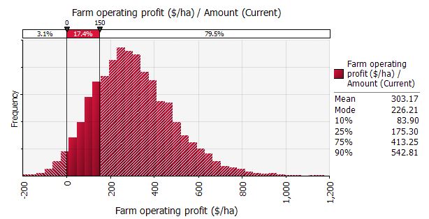
Figure 2. Farm operating profit for a 920 ha mixed cropping, sheep and cattle farm near Colac, Victoria.

The average farm operating profit (profit before financing and tax) is $303/ha. Figure 2 shows that the chances of not making a farm operating profit are very small (3.1% or one year in 32). However if this farm business had an objective to make $150/ha to service debt, pay tax and create wealth off-farm, then there is a 20.5% chance (one year in five) that this target will not be met.

While every farm is different some generalisations on the risk of different enterprise mixes can be made (based on analysis of approximately 40 mixed farms across Southern Australia).

Cropping is usually more risky than livestock

The statement ‘cropping is usually more risky than livestock’ is usually true however, risk also includes an upside as well as a downside. If the farm operating profit of the cropping and livestock enterprises are compared, the livestock operating profit has a narrower distribution, indicating there is less downside risk but also less upside potential (Figure 3).

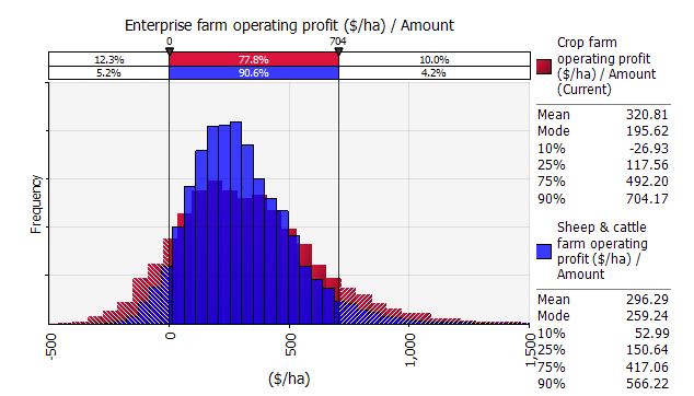
Figure 3. Net farm income from cropping (wider distribution, top numbers in legend) and livestock (narrower distribution, bottom numbers in legend).

Enterprise diversity usually decreases risk

This example illustrated in Figure 3, demonstrates that the chances of not making a profit are higher within each enterprise (12.3% for cropping and 5.2% for sheep) compared with the chances of not making a profit when the two enterprises are combined (3.3% when combined). This illustrates the effect of diversification. The benefit is that when one enterprise is going well, it offsets the losses from the other.

Identify big risks within an enterprise

The grower in this business believed cropping the marginal country was too risky and adversely affected the profit. They were considering taking the ‘marginal’ cropping land and turning it over to livestock production. A scenario was run to compare the potential impact of this change (Figure 4).

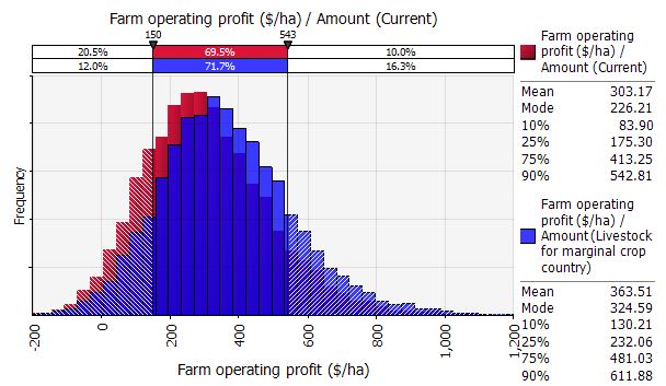
Figure 4. Farm operating profit for all cropping including the ‘marginal’ country (wider distribution, top numbers in legend) compared to only cropping the ‘good’ country and using the ‘marginal’ country to increase ewe numbers (narrower distribution, bottom numbers in legend).

Clearly the removal of the ‘marginal’ cropping country decreased the downside risk, with benefit to both the average farm operating profit and the upside risk potential. The chances of not meeting the $150/ha target has been reduced (from one year in five to one year in eight).

Other conclusions from the enterprise mix include:

• Intensification (for example by increasing stocking rate) generally increases risk.
• Sheep are usually more risky than cattle.

Conclusion

There is no single way to manage production risk. Many ‘levers’ influence the ultimate risk profile of a business and it is up to the individuals in that business to determine and feel comfortable with a level of risk that matches the rewards they seek.

Having said this, managing risk requires making decisions. The type of analysis used in Grain and Graze provides a very useful platform to inform discussion and decisions around risk.

References

Keogh M 2013, 'Global and commercial realities facing Australian grain growers' in robust cropping systems - the next step. GRDC Grains Research Update for Advisers 2013. Bendigo, Vic. pp 13-30.

Nicholson C 2013, 'Analysing and discussing risk in farming businesses’. Extension Farming Systems Journal. Vol. 9 (1) Australasia Pacific Extension Network. pp 178-182.

Useful resources

Grain and Graze 3 website

Acknowledgements

The research undertaken as part of this project is made possible by the significant contributions of growers through their support of the GRDC — the author would like to thank them for their continued support.

Contact details

Cam Nicholson
Nicon Rural Services
Grain and Graze
cam@niconrural.com.au