Economic trends and opportunities for Australian agriculture

Take home messages

• Major agricultural commodity prices are expected to remain around current levels until 2022.
• Australian interest rates are expected to start moving up next year, but in a gradual limited way.
• The value of the Australian dollar will be dictated largely by events overseas, particularly the US and China.
• Medium term economic developments in Asia will provide opportunities for Australian agriculture.

The outlook for commodity prices

Prices of Australia’s major agricultural commodity exports are expected to remain broadly stable over the next few years (Figure 1).

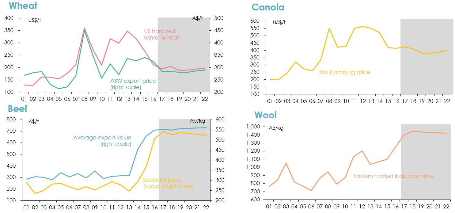
Figure 1. Historical commodity price for wheat, canola, beef and wool and their expected price over the next few years (2018-2022) (Source: ABARES).

The outlook for interest rates

The Reserve Bank’s official cash rate is the lowest it’s ever been (Figure 2).

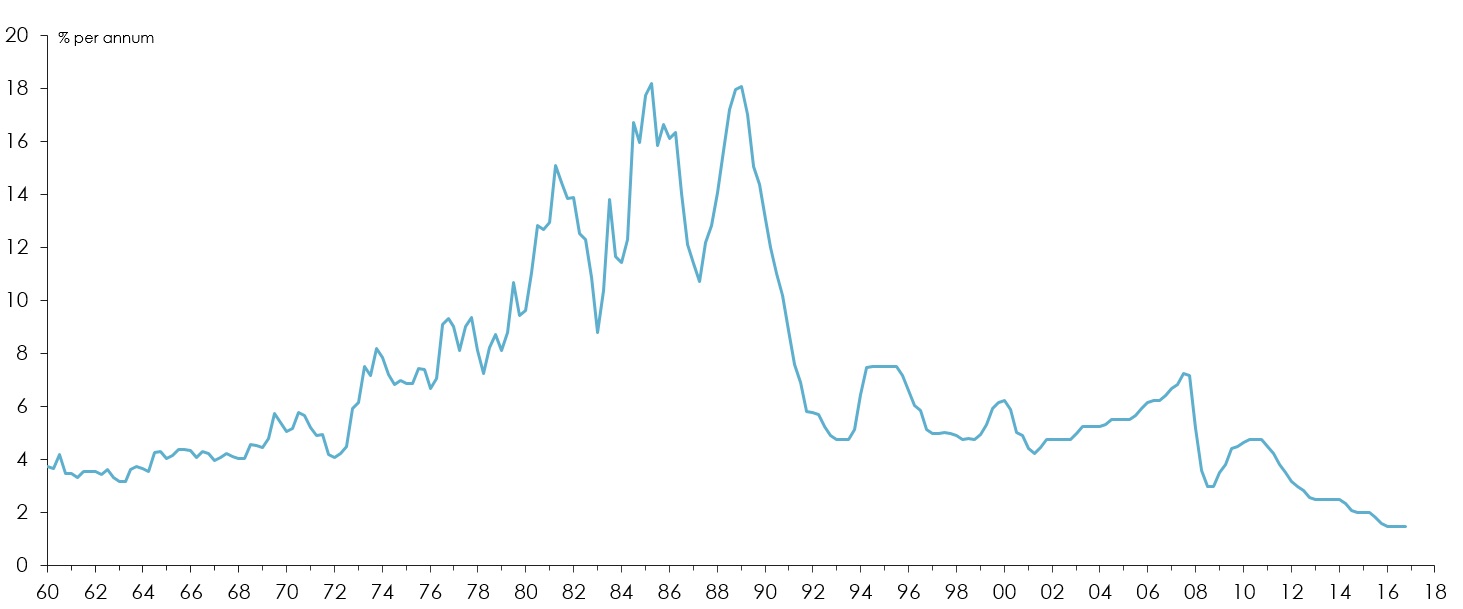
Figure 2. The Reserve Bank’s official cash rate (Source: Reserve Bank of Australia).

Interest rates actually paid on business and housing loans are also at record lows, though some rates have been rising on some housing loans (Figure 3).

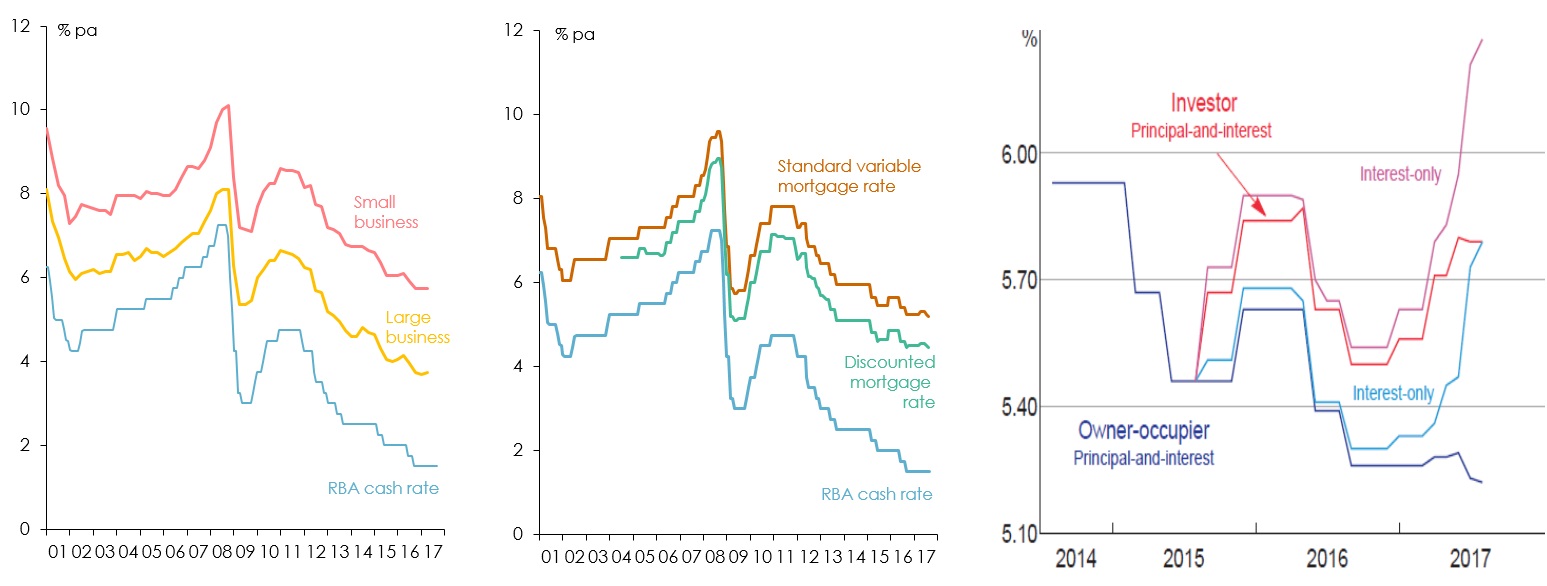
Figure 3. a) Business loan interest rates (left) b) Housing loan interest rates (centre) and c) Recent developments in housing loan interest rates (right) (Source: Reserve Bank of Australia).

Interest rates in most major overseas countries fell to even lower levels than Australia after the financial crisis, but some are now starting to rise (Figure 4).

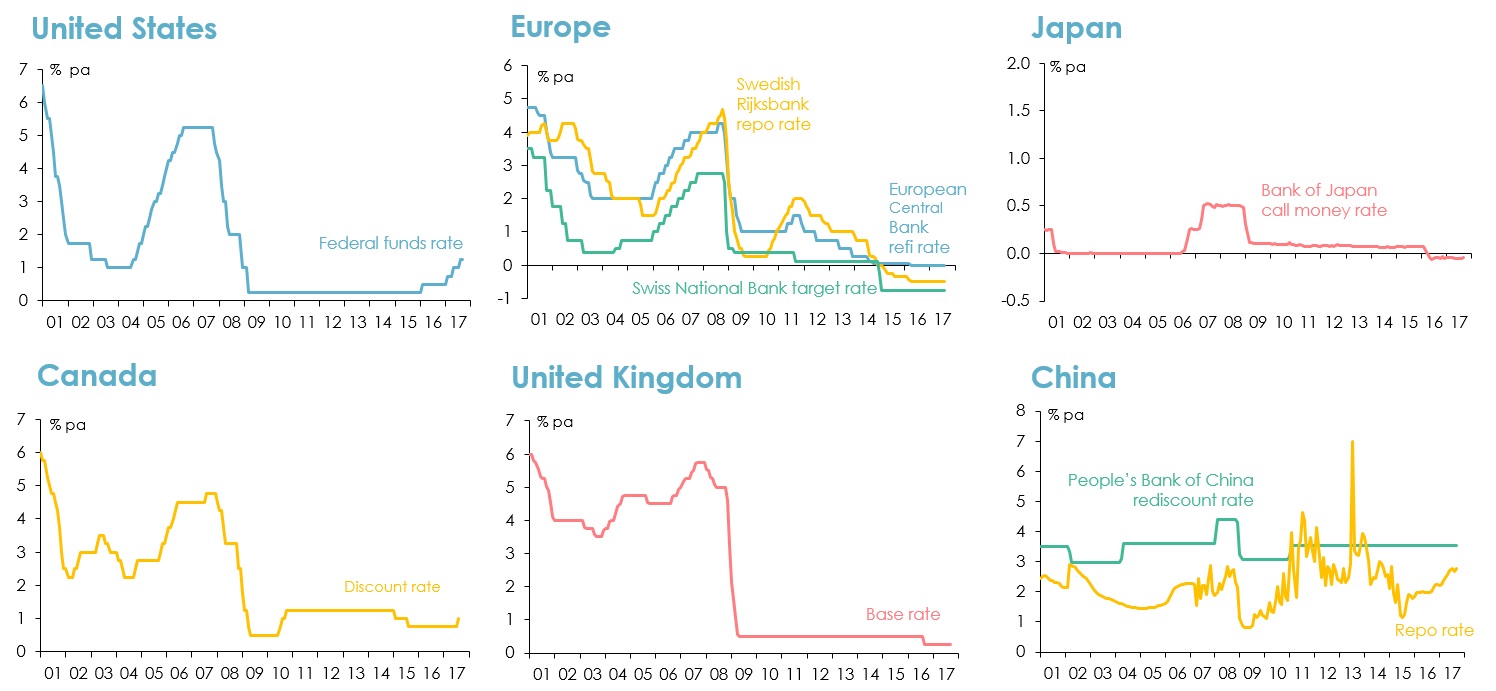
Figure 4. Interest rates in a number of overseas countries before and after the financial crisis (Sources : US Federal Reserve Board; Bank of Canada; European Central Bank; Swedish Rijksbank; Swiss National Bank; Bank of England; Bank of Japan, People’s Bank of China; Thomson Reuters Datastream).

The Reserve Bank of Australia wants to see inflation at between 2 and 3%, economic growth around 3%, unemployment at around 5% and less ‘under-employment’ (Figure 5).

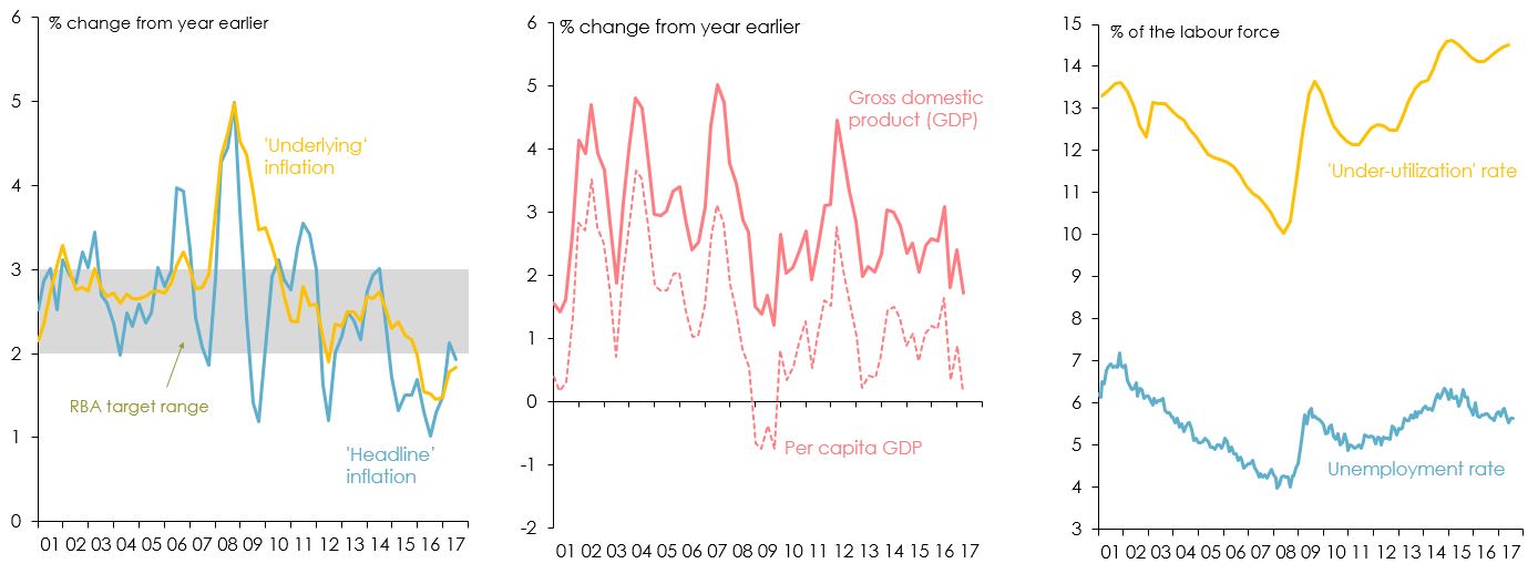
Figure 5. a) Consumer prices (left) b) Economic growth (centre) and c) Unemployment and under-employment (right) Note: ‘underlying’ inflation abstracts from the impact of volatile items (typically items such as petrol, or fruit and vegetables) on the consumer price index. The labour force ‘under-utilisation’ rate includes paper employed part-time who are willing and able to work to longer hours (and weights them equally with people who are ‘unemployed’ in the conventional sense) (Source: Australian Bureau of Statistics).

Record low interest rates have stimulated a surge in capital city house prices and a boom in dwelling construction, but also record levels of debt (Figure 6).

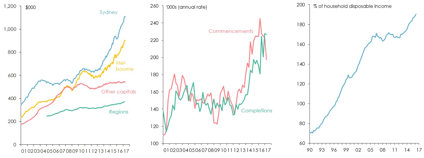
Figure 6. a) Housing prices – Sydney, Melbourne versus the rest (left) b) National housing construction rate (centre) c) Household debt (right) (Source: CoreLogic – RP Data; Australian Bureau of Statistics; Reserve Bank of Australia).

However, consumer spending and business investment – normally the two largest drivers of economic growth, have remained weak (Figure 7).

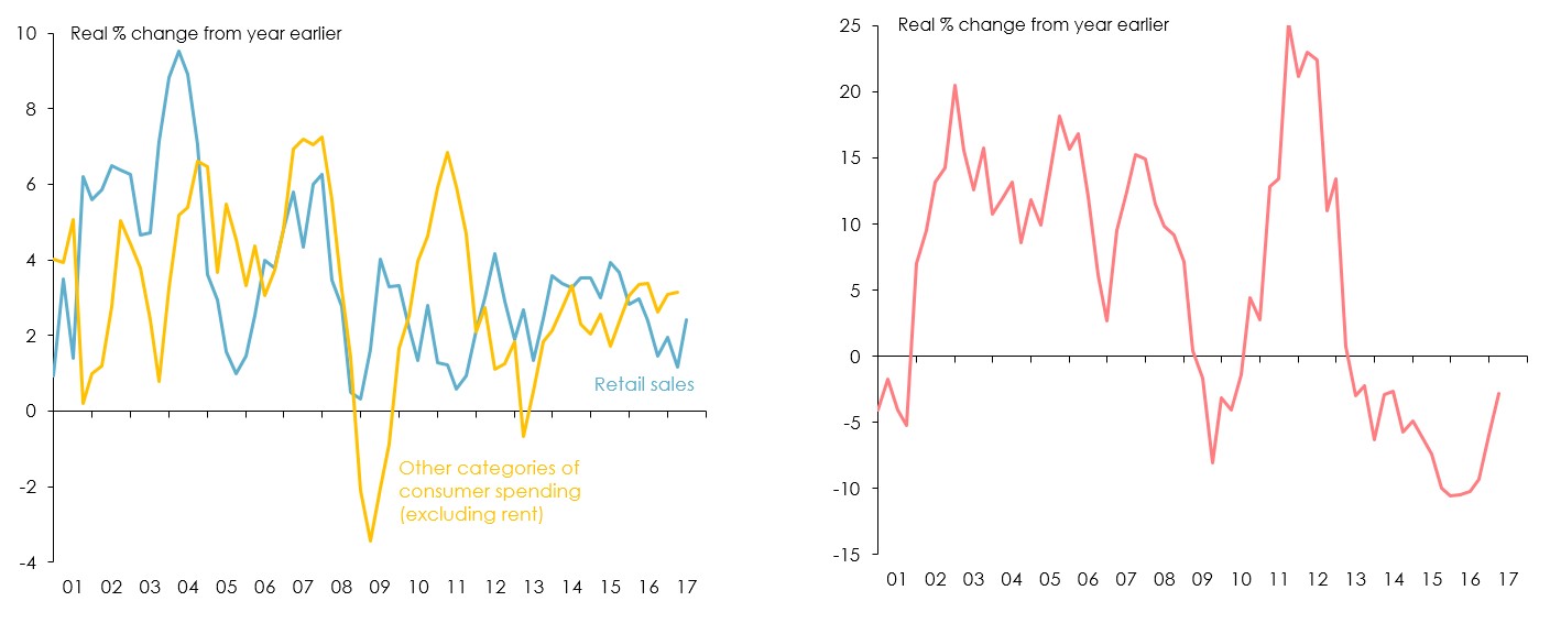
Figure 7. a) Household consumption expenditure (2001-2017) (left) b) Business investment expenditure (2001-2017) (Source: Australian Bureau of Statistics).

Sluggish growth in wages has meant weak growth in household incomes and depressed levels of consumer confidence (Figure 8).

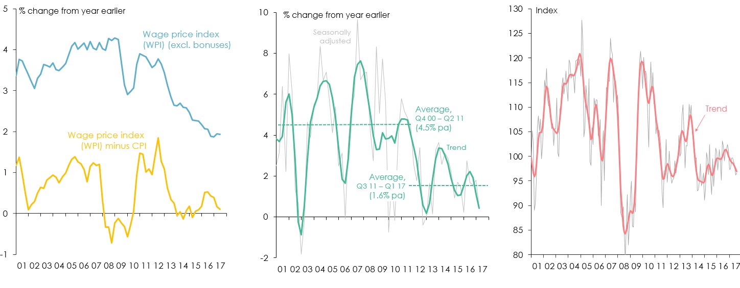
Figure 8. a) Nominal and real wages (2001-2017) (left) b) Real household disposable income (2001-2017) (centre) c) Consumer confidence (2001-2017) (right) (Source: ABS; Westpac and Melbourne Institute of Applied Economic & Social Research).

Weak growth in wages has been common among ‘advanced’ economies, especially following periods of high unemployment (Figure 9).

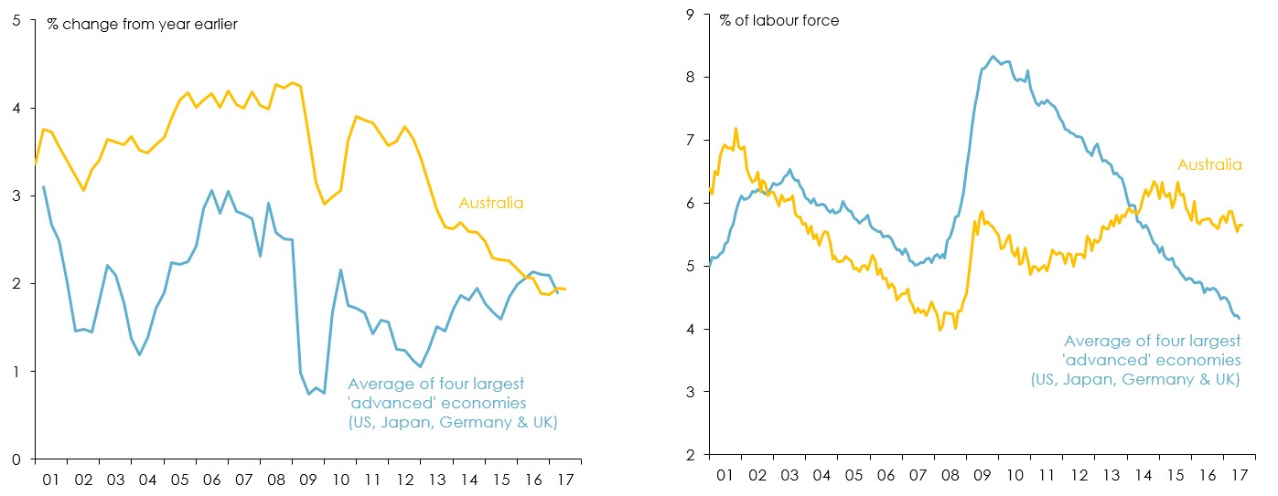
Figure 9. a) Growth in wages – Australia versus the four largest ‘advanced’ economies (2001-2017) (left) b) Rate of unemployment – Australia versus the four largest ‘advanced’ economies (2001-2017)  (right) (Source: US Bureau of Labour Statistics; Japan Ministry of Health, Labour & Welfare; Deutsche Bundesbank; UK Office for National Statistics; Australian Bureau of Statistics).

Employment growth seems likely to pick up, which should eventually be reflected in stronger wages growth (Figure 10).

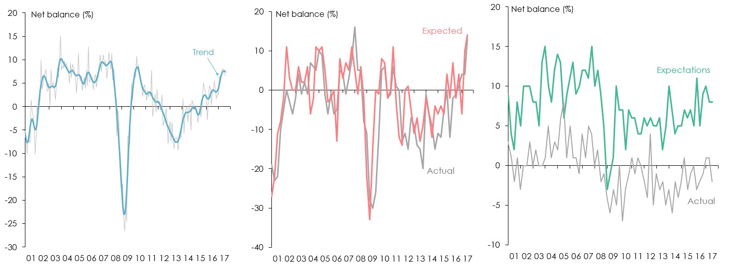
Figure 10. a) National Australia Bank survey of employer hiring intentions (2001-2017) (left) b) Westpac Australian Chamber of Commerce and Industry survey – employee numbers (2001-2017) (centre) c) Sensis SME survey – size of workforce (2001-2017) (right) (Sources: National Australia Bank; Westpac and Australian Chamber of Commerce and Industry; Sensis).

Similarly it seems likely that business investment will ‘bottom out’ and start to pick up over the next year (Figure 11).

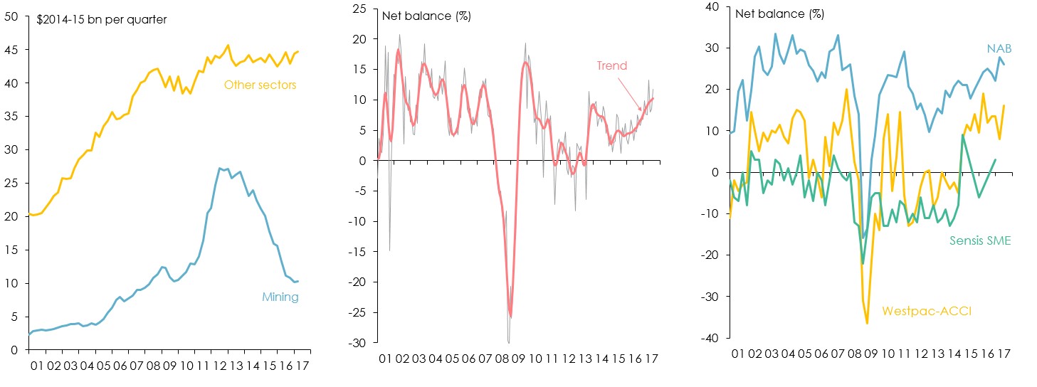
Figure 11. a) Business investment for mining and other sectors (2001-2017) (left) b) Business confidence (2001-2017) (centre) c) Business survey of capital expenditure expectations (2001-2017) (right) (Sources: National Australia Bank; Westpac and Australian Chamber of Commerce and Industry; Sensis).

Higher levels of infrastructure investment spending will also provide some impetus to economic growth (Figure 12).

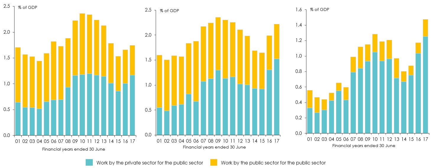
Figure 12. Indicators of engineering construction activity for the public sector: a) Value of work done (2001-2017) (left) b) Commencements (2001-2017) (centre) c) Work yet to be done (2001-2017) (right). Note: Figures for 2016-17 are for first three quarters (work done) or first half (commencements and work yet to be done) (Source: ABS).

Financial markets are expecting Australian interest rates to go up, although not very much and not very soon (Figure 13).

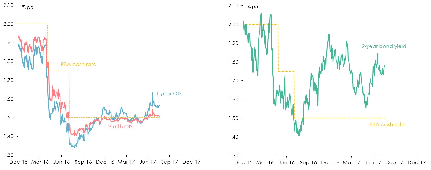
Figure 13. a) Overnight index swap (OIS) rates and the Reserve Bank cash rate (Dec 2015-Dec-2017) (left) b)Two-year Commonwealth bond yields and the Reserve Bank cash rate (Dec 2015-Dec 2017) (right) (Source: Reserve Bank of Australia; Thomson Reuters Datastream).

The outlook for the Australian dollar

The Australian dollar has been surprisingly strong against the US$ and other major currencies since mid-2015 (Figure 14).

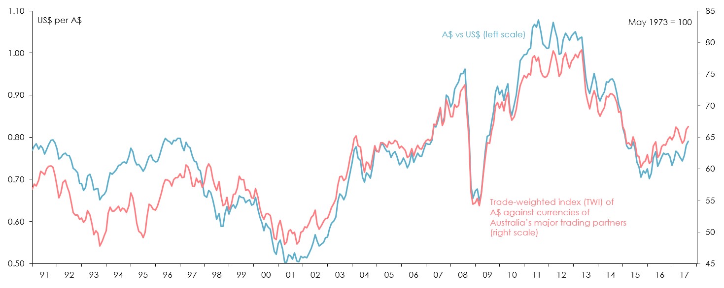
Figure 14. The Australian dollar versus the US dollar and other currencies (Source: Reserve Bank of Australia).

The unexpected resilience of the A$ against the US$ is largely the result of a surprising fall in the US$ with help from a rebound in iron ore prices (Figure 15).

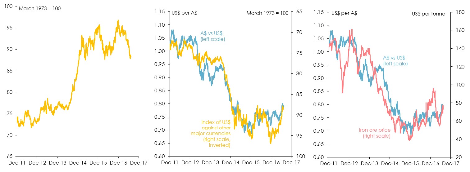
Figure 15. a) Index of US dollar against other major currencies (Dec-2011 to Dec-2017) (left) b) Australian dollar versus US dollar versus other major currencies (Dec-2011 to Dec-2017) (centre) c) Australian dollar and US dollar versus iron ore prices (Dec-2011 to Dec-2017) (right) (Sources: US Federal Reserve Board; Reserve Bank of Australia; Thomson Reuters Datastream).

US consumer and business confidence improve markedly after Donald Trump won the presidential election last November 2016 (Figure 16).

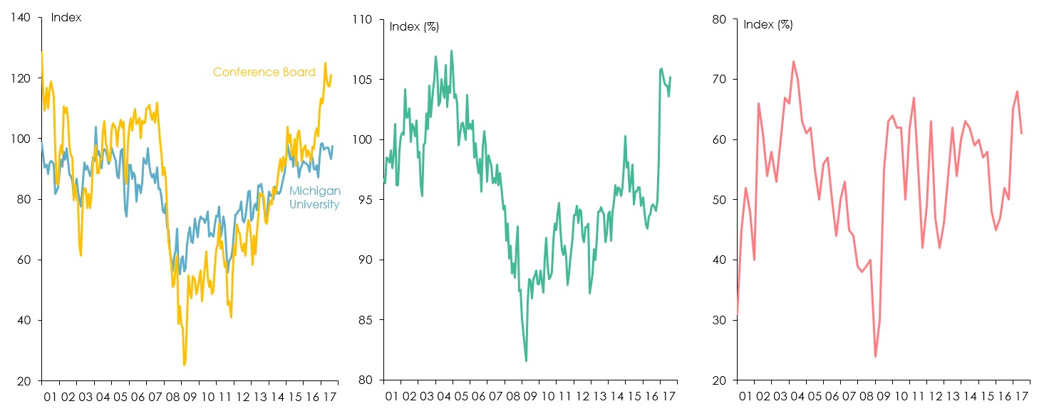
Figure 16. a) Consumer confidence (2001-2017) (left) b) Small business optimism (2001-2017) (centre) c) CEO confidence (2001-2017) (right) (Sources: The Conference Board; University of Michigan Survey Research Centre; National Federation of Small Businesses).

The share market remains optimistic about prospects for the US economy under Trump, but other financial markets are now much less convinced (Figure 17).

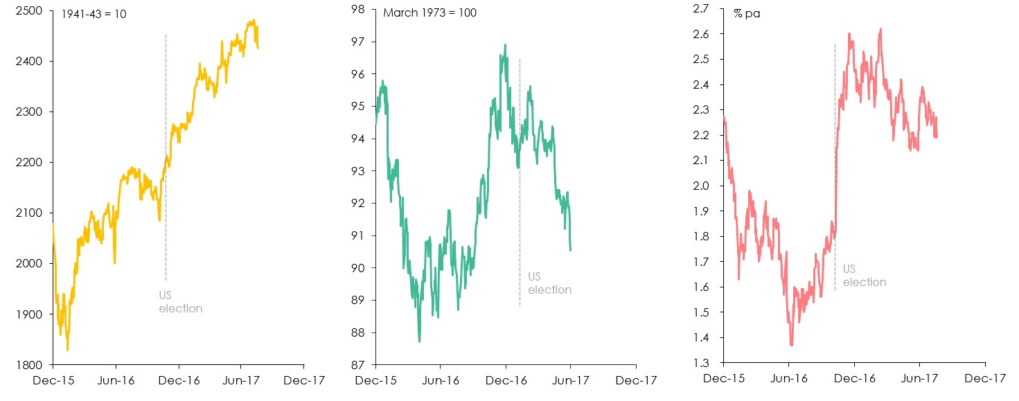
Figure 17. a) S&P 500 (left) b) US 10 year bond yield (centre) c) US dollar (right) (Source: Thomson Reuters Datastream) (Source: Thomson Reuters Datastream).

Three reasons why Trump’s fiscal policies, if they are legislated, wouldn’t have the same effect as Reagan’s (Figure 18).

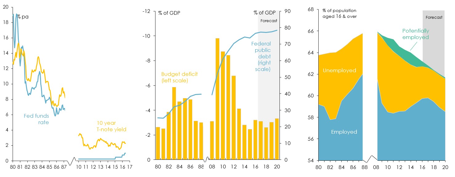
Figure 18. a) Interest rates (left) b) Federal budget and debt (centre) c) Labour supply (right) (Sources: US Federal Reserve; US Congressional Budget Office).

China’s economy is slowing, partly because its workforce has started to shrink and it also has a potentially massive debt problem (Figure 19).

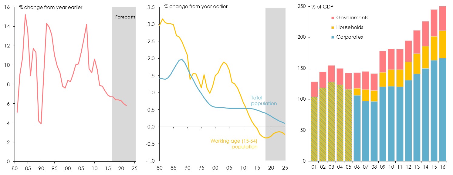
Figure 19. a) China real GDP growth (left) b) Chinese population (centre) c) Chinese debt (right) (Sources: China National Bureau of Statistics; IMF; UN Economic & Social Affairs Division, Population Branch; Bank for International Settlements).

China has been through another debt-driven property investment cycle which appears to have peaked in recent months (Figure 20).

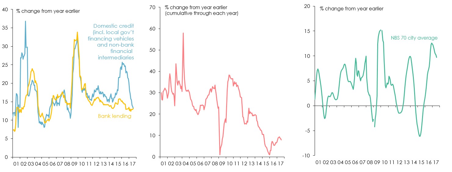
Figure 20. a) China’s credit growth (left) b) China’s real estate investment (centre) c) China’s urban property prices (right) (Sources: People’s Bank of China; China National Bureau of Statistics).

China has become more concerned about a sharp fall in its own currency – prompting it to impose tighter controls on capital outflows. (Figure 21).

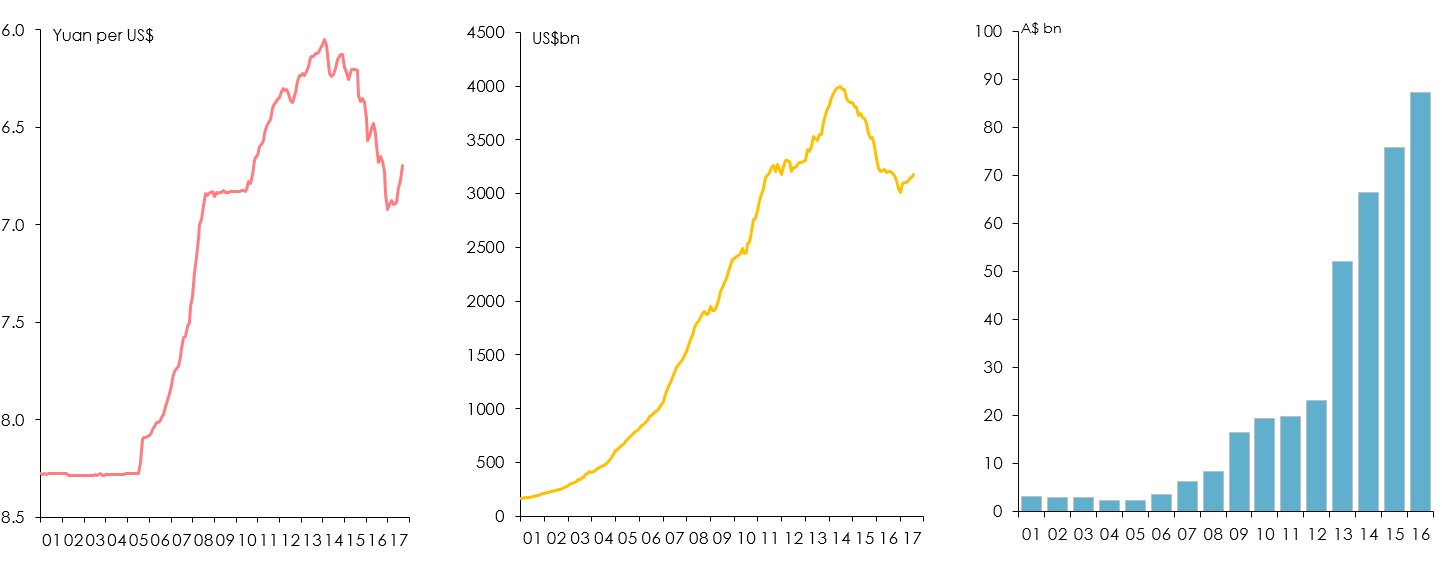
Figure 21. a) Chinese yuan versus US$ (left) b) China’s foreign exchange reserves (centre) c) Chinese foreign investment into Australia (right) (Sources: People’s Bank of China; Australian Bureau of Statistics).

Longer term prospects for Australian agriculture

The numbers and spending power of ‘Asian middle classes’ will increase dramatically over the next 15 years (Figure 22).

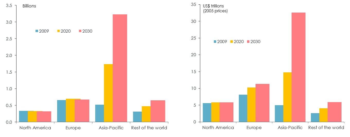
Figure 22. a) Numbers of ‘middle class’ consumers (left) b) ‘Middle class’ consumer spending (right). Note: ‘Middle class’ is defined as people with daily spending of between US$10 and US$100 in 2005 prices converted at purchasing power parity exchange rates. (Source: Homi Kharas and Geoffrey Gertz, ‘The New Global Middle Class: A Cross-Over from West to East’, Wolfenshohn Centre for Development, The Brookings Institution, Washington DC, 2010).

However Asia’s potential to lift agricultural production is limited by constraints on both land and water (Figure 23).

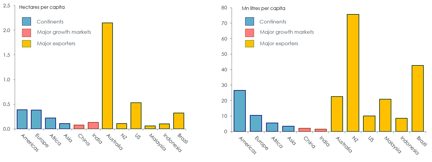
Figure 23. a) Hectares per capita of arable land (left) b) Million litres per capita of renewable water supply (right) (Source: ANZ & Port Jackson Partners, Greener Pastures: The Global Soft Commodity Opportunity for Australia and New Zealand, October 2012).

So the growth rate of agricultural production is likely to slow – especially in Asia (Figure 24).

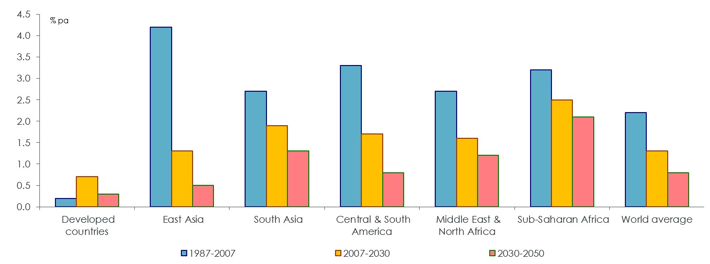
Figure 24. Growth rates in agricultural production (Source: Nikos Alexandratos & Jelle Bruinsma, World Agriculture Towards 2030/2050: The 2012 Revision, ESA Working Paper No 12-03, Food and Agriculture Organisiation (June 2012).

Asian countries (in particular) will need to import a lot more food products (Figure 25).

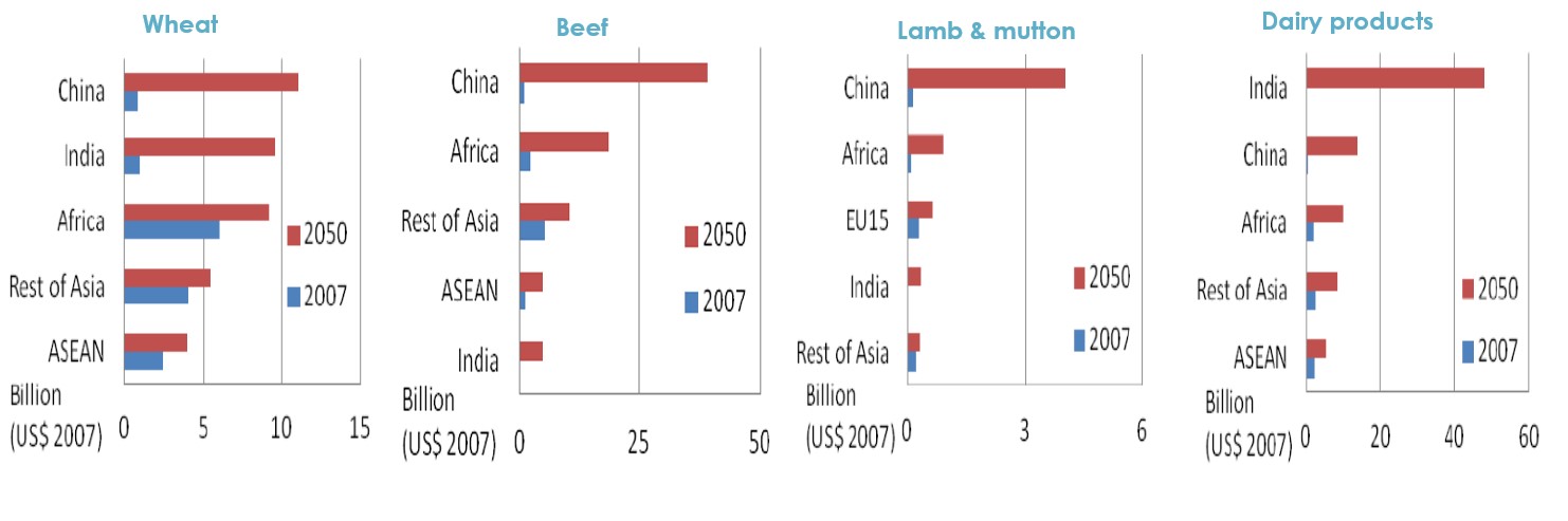
Figure 25. Sources of global food (wheat, beef, lamb & mutton, and dairy products) (Source: Verity Linehan, Sally Thorpe, Neil Andrews, Yeon Kim & Farah Beaini, Food Demand to 2050: Opportunities for Australian Agriculture, Paper presented to 42nd ABARES Outlook Conference, 6-7 March 2012; Australian Government, Australia in the Asian Century White Paper, October 2012).

However to capitalise on that opportunity, Australian agriculture will need to improve its productivity (Figure 26), adapt to climate change (Figure 27) and attract new capital investment (inevitably) including from foreign sources (Figure 28).

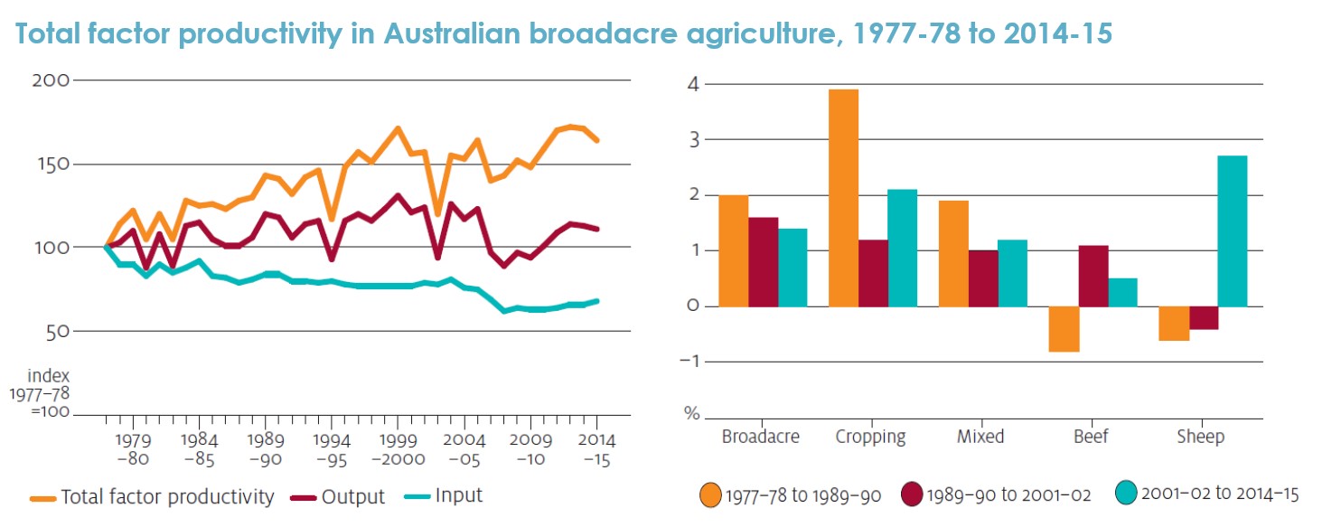
Figure 26. Total factor productivity in Australian broadacre agriculture, 1977-78 to 2014-15. Note: Total (or multi-) factor productivity is the ratio of total production to a measure of inputs (land, labour, capital and materials & services) used in the production process (Source: Charley Xia, Shiji Zhao and Haydn Valle, ‘Productivity in Australia’s broadacre and dairy industries’ in Agriculural Commodities, ABARES, March 2017).

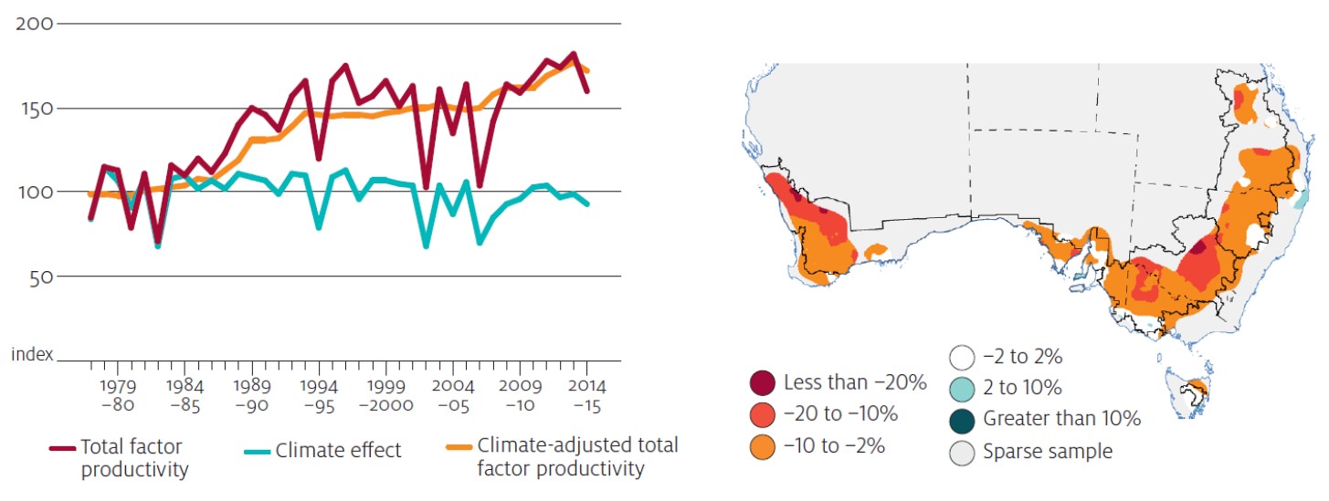
Figure 27. Impact of climate change on productivity levels in cropping (Source: Neal Hughes, Kenton Lawson and Haydn Valle, Farm performance and climate: climate-adjusted productivity on broadacre cropping farms, ABARES, May 2017).

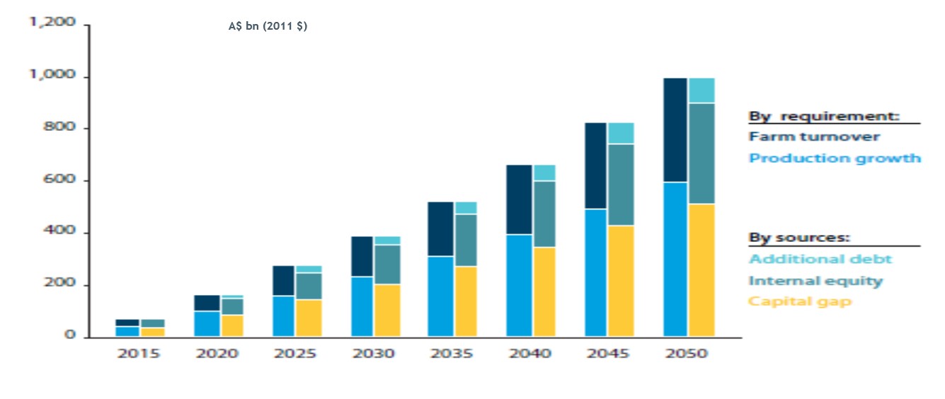
Figure 28. Cumulative capital required by the Australian agricultural sector (Source: ANZ & Port Jackson Partners, Greener Pastures: The Global Soft Commodity Opportunity for Australia and New Zealand, October 2012).

Conclusion

• Major agricultural commodity prices to remain around current levels.
  • Subject to the usual risks around major weather events, natural disasters and big shifts in trade policies.
• Australian interest rates will start moving up next year – but in a gradual, limited way.
  • The RBA does not want to cut rates any further (unless there is a major adverse economic shock) for fear of further stoking metropolitan property prices and household debt.
  • But nor does it want to start raising them until it is much more confident that inflation is back within its 2-3% target range and unemployment is closer to 5%.
  • The timing of any changes in the RBA’s interest rates won’t be dictated by movements in overseas rates.
  • Interest rates will not rise by very much over the next few years.
• The Australian dollar’s fortunes will be dictated largely by events overseas, particularly the US and China.
  • If the US$ continues to weaken, then the A$ will stay uncomfortably high (for exporters).
  • But if by some chance Trump does get his act together and the US economy strengthens, the A$ will fall back to the low US70s.
  • A ‘hard landing’ in China would almost certainly send the A$ into the US60s.
• Medium term economic developments in Asia provide opportunities for Australian agriculture.
  • However Australian agriculture will face a lot more competition than Australian mining.
  • Australian agriculture will need to improve productivity and attract more investment capital.

Contact details

Saul Eslake
saul.eslake@gmail.com