Statistics 101 and making it sexy
Author: Dale Grey (Agriculture Victoria, Bendigo) | Date: 26 Feb 2019
Take home messages
- The p value needs to be less than 0.05.
- It is good if the CV% is less than 10%.
- Values must be greater than the LSD apart to be significant.
- Always ask for statistical analysis.
Background
For many first-year science graduates, even more so than chemistry or physics, statistics was the particular subject that many found the hardest to grasp. So, it is not surprising that statistical knowledge is something that people either try to avoid or they use it in error. The problem is that agriculture often consists of scientific trials and data presentations that require a rudimentary knowledge of statistics to be understood properly.
Discussion
Number of observations
These are a couple of letters I like to see in all data presentations i.e. how many observations are in the data set where comparisons are being made. This is particularly important in survey data as often there is no replication. The conclusions where n=24 could be much more meaningful if n=240 or n=2400. In other words we should have greater confidence in result findings when data is collected in greater numbers, or on the flip side greater caution if the dataset is small.
Replication
Replication or reps (sometimes called blocks) is also a critical number. Is there - none?, three?, eight?. The data analysis validity is backed up by the amount of replication. In agricultural experiments, three is usual, four is better, two is dicey. In laboratory-based trials of pots or agar plates, higher replication numbers are common. Because we are dealing with science and not the arts, replicates help to overcome the possibility that each applied treatment does not behave in a uniform way, usually for reasons unknown. Trial managers are always on the lookout for the ‘mythical’ area of uniform soil type. My experience in Victoria is they are very hard to find. All is not lost though. If your trial goes from light to medium to heavy soil, do not run the replicates down the variation so that every replicate has a bit of each soil type. Run your replicate along similar soil type so that each treatment in the replicate has the same soil type effect. Similarly, for slope, stubble density, and spray wheel track.
P value
In trials analysed by Analysis of Variance (ANOVA), the whole point of the analysis is to find the probability that the data is not all the same. In other words, what is the probability that there is something significant happening in the data? The p value tells the probability of all of our data being statistically similar. P values for agricultural research are often set at 0.05 or 5% or less i.e. for something to be considered statistically significant, there has to be only a 5% chance of the numbers being the same. Some fields of research might accept 0.1 or 10%, others might want to be more emphatic and require 0.01 or 1% or 0.001 or 0.1%. Once it was common to allocate *’s to the significance level, 0.05 =*, 0.01=**, 0.001=*** of significance. Old journal papers often used this system. The major school of statistical thought says that if there is no significance in the ANOVA then you are not entitled to present an LSD value, even if that LSD can show a difference in the data. Use of the terms ’a trend towards’, ’a suggestion of’ should indicate that the data has not met the 0.05 level.
ANOVA has some important rules for use that often are ignored. The major one is that the data must be distributed normally. When the data range is plotted, it should look similar to Figure 1.

Figure 1. Graph of a normal distribution showing the mean and +/- 2 to 3 standard deviations from the mean.

Figure 2. Soybean yield histogram showing normally distributed data, n=21.
Every fundamental of an ANOVA is based on the data being normalised or else some other statistical technique must be used. If the data does not normalise, then transformations of the data using log, arcsin or some other statistical means might be needed to make it normally distributed - it might be time to seek professional statistical advice. Experience has told me to never score plots with yes/no categories as this data is often not being normally distributed. It is always best to use a scale of 1-5, 1-10 or similar. However, scoring data is often problematic. For example, with data such as rust, lodging or head loss, the majority of the data is often at one end of the rating scale (i.e. only a few resistant varieties and everything else susceptible), making it not normally distributed.
Coefficient of variation percentage
The coefficient of variation percentage or CV% is a measure of how variable the data set is around the average. It is calculated by dividing the standard deviation by the mean. The larger the variability in the data, the higher the CV% — if the data points are all the same then the CV% is zero. If there are large differences in the numbers in the data set, it could be close to 100%. The CV% can be calculated for a whole trial, within replicates or across replicates, each indicating something about the variation of the site and the treatments.
To demonstrate the effect data spread has on the CV%, consider the following three data sets:
46, 47, 50, 52, 55 has an average of 50, a standard deviation of 3.7 and a CV% of 7.3.
40, 45, 50 ,55, 60 has an average of 50, a standard deviation of 7.9 and a CV% of 15.8.
20, 40, 50, 60, 70 has an average of 50, a standard deviation of 15.8 and a CV% of 31.6.
In cereal and canola trials, a CV% between 0-10% is considered desirable, while less than 5% is best. Values higher than 15% often indicate an unreliable trial and should be treated with caution — in the instance of the NVT database, they are deleted from analysis. Pulse crops are generally more variable and values such as 10%-15% might be deemed suitable for the lack of anything better.
Least significant difference
The least significant difference (LSD) number is a different metric to the p value that is used to indicate the significance between data values (the p value only indicates that there is a difference somewhere in the data but not exactly what it is). LSD is often quoted with a probability value as well, often at the 0.05 or 5% level, but like p values, LSD can be seen at higher or lower levels of confidence. Higher probability LSDs may mean the author is ’fishing’ for significance, but it can be frustrating if your treatment effect is significant at the 6% level — usually the author should state if and why they have deviated from an LSD of 5%.
In brief, if two data values are greater than the LSD apart, then there is only a 5% chance that they can be statistically the same. If the difference is equal to the LSD, it is not significant at the 5% level. For a simple trial where variety is the treatment, the LSD quoted simply shows which yields are statistically the same and which are not. More complex trials such as rate experiments might often show an LSD for the whole trial, and for individual treatment means. This is often where statistical communication breaks down —when the treatment means are not presented and you are supposed to work them out in your head.
Table 1 shows the mean data for a whole experiment and includes all ANOVA analysis for both p value and LSD for comparison across all treatments and the interactions between treatments. Obviously, such a table can be difficult to interpret. All that the analysis shows is that sowing width and variety are significant and nothing else is. Often people will only include that analysis and disregard the others. The use of the * holds a special significance in ANOVA treatment descriptions as it is called the interaction. It looks for statistical significance in combinations of treatments that are different to the mean of the treatments by themselves. In my experience, interactions are rare, however they sometimes happen.
Table 1a. Sowing rate x sowing width x varieties soybean yield trial.
Density | 35p/m2 | 50p/m2 | |||||||
Width | 96248-23 | Djakal | Snowy | 96248-23 | Djakal | Snowy | |||
35cm | 4.09 | 5.09 | 4.58 | 4.29 | 5.25 | 4.72 | |||
70cm | 2.97 | 3.98 | 3.51 | 3.33 | 3.96 | 3.57 | |||
mean | 4.11 | ||||||||
CV% | 9.9 | ||||||||
p Width | <.001 | LSD Width | 0.24 | ||||||
p Rate | 0.21 | LSD Rate | 0.24 | ||||||
p Variety | <.001 | LSD Variety | 0.29 | ||||||
p Width*Rate | 0.89 | LSD Width*Rate | 0.34 | ||||||
p Width*Variety | 0.85 | LDS Width*Variety | 0.41 | ||||||
p Rate*Variety | 0.73 | LDS Rate*Variety | 0.41 | ||||||
p Width*Rate*Variety | 0.83 | LSD Width*Rate*Variety | 0.58 | ||||||
Such a large number of statistics can be summarised in a much simpler way, clearly showing 35cm rows yielding statistically higher than 70cm and each variety statistically significant in yield from each other (Table 1b and 1c)
Table 1b. Sowing width x soybean yield trial.
| Width | Yield |
|---|---|
| 35cm | 4.67 |
| 70cm | 3.55 |
| mean | 4.11 |
| CV% | 9.9 |
| p | <.001 |
| LSD 5% | 0.24 |
Table 1c. Varieties soybean yield trial.
| Variety | Yield |
|---|---|
| Djakal | 4.57 |
Snowy | 4.10 |
| 96248-23 | 3.67 |
| mean | 4.11 |
| CV% | 9.9 |
| p | <.001 |
| LSD 5% | 0.29 |
Another way of showing significance between data is the lettering system. Here the term ’treatments containing different letters denote statistical significance’ usually appears. This data presentation method has worked out all significant data by placing different letters after them. However, it is better used for smaller numbers of comparisons rather than larger ones, otherwise it becomes too cumbersome. In the example in Table 2, the term variety F148-4 ’topped the trial’ is often heard — it may well have, but it is actually not statistically significant to all the varieties below it until F191a-4 is reached. All varieties until then have an ’a’ after them denoting they are statistically the same. A correct statement is variety F148-4 yielded statistically higher than F191a-4, but not higher than anything between those two varieties. Similarly, all varieties with a ’c’ code are the same and so Djakal was statistically higher yielding than Snowy.
Table 2. Soybean variety trial using letter codes for LSD significance.
| Variety | Yield |
|---|---|
| F148-4 | 3.46a |
| 99091A-4 | 3.29ab |
| Djakal | 3.21abc |
| F215-9 | 3.16abcd |
| Empyle | 3.13abcde |
| F191a-4 | 2.80bcdef |
| 96248-23 | 2.63cdef |
Snowy | 2.60def |
| F191B-4 | 2.54ef |
| F157-2 | 2.46f |
| 99024-76 | 2.41f |
| Mean | 2.88 |
| CV% | 12 |
| p | 0.01 |
| LSD 5% | 0.59 |
R2
The R2 value is often presented on a graph to explain what percentage of a fitted line or function matches the data. Theoretically, if the data perfectly matched the line of best fit, the R2 would be 100%. Good or bad R2s are a bit arbitrary as it depends on what is done with the data afterwards. For simple linear lines of best fit, a larger R2 is nearly always desirable. Simple rules of thumb are where the line might be used to make predictions for farm management and precision is not important, an R2 above 50% might be fine. If precision is required from a modelled line of best fit for making decisions, an R2 > 80% may be desirable. In psychology, an R2 below 50% is as good as it gets, because humans are not as predictable as natural systems. In statistical regression analysis which attempts to match a line to the data, it is possible to have statistically significant parameters around the line of best fit, but still have a poor R2. It is possible to have a good R2 from some data, but still have a line of best fit that grossly overestimates or underestimates small or large values put into the model, perhaps rendering it useless for practical purposes.
REML and the National Variety Testing (NVT)
Individual location NVT trial site data are analysed by ANOVA and provide p value, CV% and LSD. Combined site data or regional analysis (multi-environment trials (MET)) are undertaken using residual maximum likelihood (REML). To the uninitiated, REML is the ‘black box of statistics.’ REML has to be carried out by a competent statistician. The statistician applies simple and complex models to best explain a set of transformed data, and the best model then is used to analyse the data. The model can then also be used to predict data, sometimes where it was not actually tested. REML is an incredibly powerful tool as it can be used for data that is not normally distributed, trial designs that are unbalanced, data that has variability within the replicate and across sites that might be differently designed experiments. Trust is required when looking at REML analysed data — trust that the statisticians have done the best they can. REML was invented by Australians and has stood the test of time as a legitimate, but complex statistical technique.
A caution on the economic analysis of data
At a field day in my first year as an agronomist, I presented statistically analysed data of a nitrogen trial and the associated gross margins of the mean treatment data. A learned agronomist approached me afterwards and advised me that if there was no statistical difference in some of my treatments I was not entitled to make an economic assessment as if there were. I have never forgotten this. The bottom line is that for minimal extra work you can create a gross margin for each data point and do a full statistical analysis of the economics — sadly it is very rare to see this. Economic analysis needs to also stand up to statistical inquisition.
Gruen for agronomists
Read the scale of graphs
The major point is to include the full range of data (including zero) on the vertical axis. If you don’t, the graph might show differences that are not actually there. This can be easily tested if an LSD is provided. The graphs in Figure 3 show the same data, but with a changed scale. Sometimes this can be justified for ease of reading, but if there is no LSD value, the data may or may not be significant.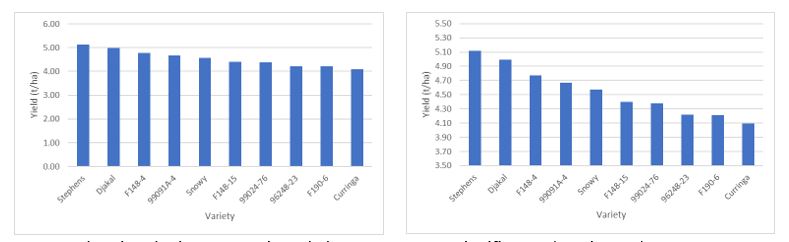
Figure 3. Showing the impact Y axis scale has on apparent significance (LSD is 0.75).
Exclusion of nil control
This trick of excluding nil control fools you into thinking that a treatment is as good as another, but failure to include the nil control could demonstrate that doing nothing was just as useful.
The following trial shows that all four methods of Rhizobia inoculation were statistically similar — a good result.
Table 3. Soybean inoculation trial with and without the control.
| Method | Yield | Method | Yield |
|---|---|---|---|
| liquid | 4.26 | liquid | 4.26 |
freeze dried | 4.16 | freeze dried | 4.16 |
granules10 | 3.90 | control | 3.96 |
peat slurry | 3.86 | granules10 | 3.90 |
peat dust | 3.85 | peat slurry | 3.86 |
granules5 | 3.52 | peat dust | 3.85 |
granules5 | 3.52 | ||
mean | 3.93 | mean | 3.93 |
p= | 0.01 | p= | 0.01 |
CV% | 6.9 | CV% | 6.9 |
LSD 5% | 0.48 | LSD 5% | 0.48 |
Inclusion of the nil control shows that this trial site was an unresponsive site to rhizobia and the existence of a background population was enough to nodulate the crop.
If there is no data presented for a nil control, ask why.
Significance by omission
At its worst, significance by omission might be because it is handpicked data not including the whole data set, leaving out current industry leading varieties, leaving out sites that tell a different story, or just omitting the data that yielded higher than a particular point. The NVT website is a good place to visit for yield data that includes all varieties at all sites. Table 4 contains two sets of data, one showing that Snowy is a high yielding variety and the other two varieties, Stephens and Djakal, also yielded similarly. Beware statistics with omissions. This is one of the most common ways of manipulating data until it shows what you want it to say. It can also be the hardest to detect.
Table 4. Soybean yield trial showing omission of higher yielding varieties.
Variety | Yield | Variety | Yield |
|---|---|---|---|
Stephens | 5.12 | ||
Djakal | 4.99 | ||
| F148-4 | 4.77 | ||
| 99091A-4 | 4.66 | ||
Snowy | 4.57 | Snowy | 4.57 |
96248-23 | 4.22 | 96248-23 | 4.22 |
F190-6 | 4.21 | F190-6 | 4.21 |
Curringa | 4.09 | Curringa | 4.09 |
F169-41 | 3.98 | F169-41 | 3.98 |
F169-34 | 3.98 | F169-34 | 3.98 |
Empyle | 3.90 | Empyle | 3.90 |
| F215-9 | 3.89 | F215-9 | 3.89 |
F191A-4 | 3.69 | F191A-4 | 3.69 |
F157-2 | 2.92 | F157-2 | 2.92 |
| F170-6 | 2.81 | F170-6 | 2.81 |
| mean | 3.97 | mean | 3.97 |
| F Prob | <0.001 | F Prob | <0.001 |
| CV% | 7.82 | CV% | 7.82 |
| LSD 5% | 0.75 | LSD 5% | 0.75 |
Conclusion
This paper has hopefully provided you with a basic understanding of how data should be presented and interpreted correctly. Important also to remember to seek trained professional advice when in doubt.
Contact details
Dale Grey
PO Box 3100 Bendigo DC 3554
0354304444
dale.grey@ecodev.vic.gov.au
@eladyerg
Was this page helpful?
YOUR FEEDBACK